Coupled Temperature - SimFlow (OpenFOAM) Description
Coupled Temperature is a boundary condition designed for conjugate heat transfer (CHT) simulations involving multiple regions, such as fluid-solid interfaces. It couples the temperature and heat flux across patches, accounting for conductive and radiative heat transfer. The condition ensures continuity of temperature and balances the heat fluxes, including optional thermal resistance layers.
The heat flux balance at the interface is given by:
- \(Q_s\) - conductive heat flux from solid region
- \(Q_{rads}\) - radiative heat flux from solid region
- \(Q_f\) - conductive heat flux from fluid region
- \(Q_{radf}\) - radiative heat flux from fluid region
This boundary condition is particularly useful in multi-region solvers like chtMultiRegionFoam.
Coupled Temperature - SimFlow (OpenFOAM) Understanding Coupled Temperature
The Coupled Temperature enforces thermal equilibrium at the interface between two regions by ensuring continuity of temperature and total heat flux (conductive plus radiative). It uses a mixed boundary condition where the interface temperature is a weighted average based on the thermal conductivities of the adjacent regions. The weighting is harmonic, giving more influence to the region with higher thermal conductivity.
The value fraction (how much the boundary value is fixed vs. gradient) is calculated as:
- \(\kappa\) - thermal conductivity of the local region
- \(\kappa_{nbr}\) - thermal conductivity of the neighbor region
The reference value for temperature is the weighted average:
- \(T\) – internal temperature of the local region
- \(T_{nbr}\) – temperature of the neighbor region
For the gradient, it accounts for source heat fluxes (e.g., Joule heating) and radiative fluxes if specified:
- \(q_s\) – source heat flux \([\frac{W}{m^2}]\)
- \(q_r\) – radiative heat flux \([\frac{W}{m^2}]\)
Optional thermal resistance layers (e.g., thin walls) are included by adjusting the effective thermal conductivity. Radiation is handled by coupling with radiative flux fields (qr), ensuring the total heat balance includes both conduction and radiation.
Coupled Temperature - SimFlow (OpenFOAM) Application & Physical Interpretation
The Coupled Temperature is used in conjugate heat transfer simulations where heat transfer occurs between different materials or phases, often including radiation effects.
Coupled Temperature in Heat Exchangers applications
Example applications: heat exchangers, boilers, furnaces
This problem can be solved using chtMultiRegionFoam (solver). The Coupled Temperature is applied at solid-fluid interfaces to couple temperature and heat flux.
| Physics | Temperature | Radiative Flux | Radiation |
|---|---|---|---|
Solid Region Interface | Coupled Temperature | Calculated | Radiation |
Fluid Region Interface | Coupled Temperature | Calculated | Radiation |
| Tutorial | Description |
|---|---|
Simulates heat transfer between hot and cold regions in a heat exchanger with separate flows, using thermal resistance to model conduction through a single boundary. | |
Solves the conjugate heat transfer problem for a plate exposed to heat from equipment, analyzing fluid circulation for efficient heat dissipation. |
Coupled Temperature in Electronics Cooling applications
Example applications: electronic devices, CPUs, circuit boards
Using chtMultiRegionSimpleFoam (solver) for steady-state simulations. The Coupled Temperature models heat dissipation from hot components to coolant.
| Physics | Temperature | Radiative Flux | Radiation |
|---|---|---|---|
Solid-Fluid Interface | Coupled Temperature | Calculated | Radiation |
| Tutorial | Description |
|---|---|
Models electronic cooling with Joule heating in a CPU and conjugate heat transfer at the interface with flowing air. |
Coupled Temperature - SimFlow (OpenFOAM) Coupled Temperature in SimFlow
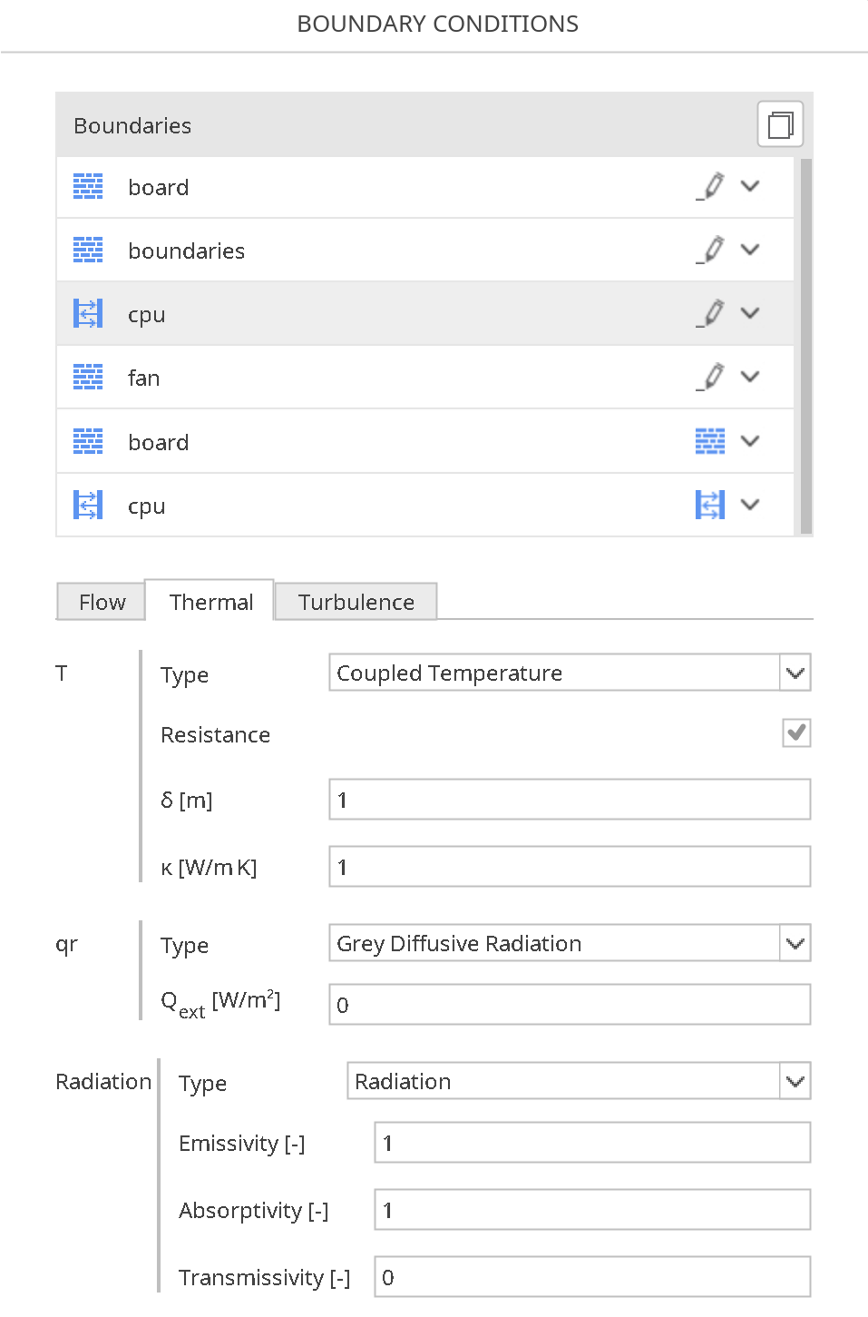
The definition of boundary conditions in SimFlow is both simple and intuitive. To specify the Coupled Temperature boundary condition, the user must navigate to the Boundary Conditions panel, select the appropriate interface boundary. In Thermal tab, choose the correct option from the drop-down menu.
For temperature fields in multi-region setups, select Coupled Temperature.
Parameters include: - Resistance: Enable/disable thermal resistance layer - \(\delta\): Thickness of resistance layer - \(\kappa\): Thermal conductivity of resistance layer - \(q_{rad}\): Radiative heat flux - Radiation properties: Emissivity, Absorptivity, Transmissivity
Parameters include:
Resistance - Enable/disable thermal resistance layer
\(\delta\) - Thickness of resistance layer
\(\kappa\) - Thermal conductivity of resistance layer
Coupled Temperature - SimFlow (OpenFOAM) Coupled Temperature - Alternatives
In this section, we propose boundary conditions that are alternative to Coupled Temperature. While they may fulfill similar purposes, they might be better suited for a specific application and provide a better approximation of physical world conditions.
| Boundary Condition | Description |
|---|---|
Similar to Coupled Temperature but without radiation effects, suitable for pure conductive heat transfer. |