Fixed Gradient - SimFlow (OpenFOAM) Description
Fixed Gradient also known as the Neumann or Second-Type boundary condition, specifies a gradient normal to the boundary (perpendicular to the boundary face):
- \(\phi\) is the scalar or vector field
- \(\nabla \phi\) is the gradient of the field
- \(\mathbf{n}\) is the normal vector to the boundary
Often, the specified gradient is zero, which corresponds to Zero Gradient boundary condition.
In the Fixed Gradient boundary condition, the gradient of the scalar or vector field on the boundary is set to a specific constant value. This configuration permits the field’s value to vary across the boundary, but the rate of change, or gradient, remains fixed.
The gradient of a quantity is often related to a diffusive flux. For example, in heat transfer problems, the gradient of temperature multiplied by the thermal conductivity denotes the heat flux (Fourier’s law of heat conduction).
Fixed Gradient - SimFlow (OpenFOAM) Understanding Fixed Gradient
To have a better understanding of how the Fixed Gradient works, let’s consider a 1D grid. The gradient \(\frac{d\phi}{dx}\) can be discretized at two neighboring points \(x_{i}\) and \(x_{i+1}\) using finite difference in the following way:
- \(\phi_{i}\) and \(\phi_{i+1}\) are the values of \(\phi\) (dependent variable) at \(x_{i}\) and \(x_{i+1}\), respectively
- and \(\Delta x\) is the grid spacing
Given the Fixed Gradient boundary condition:
From the equation above, we can read that the boundary condition enforces only a fixed difference between the neighboring cells, while the value of the solution at the boundary depends on results further away, inside the domain. Thus, this condition allows us to control how fast the solution changes across the boundary, but not the solution values themselves.
Inlet Flux
The generic inlet flux \(J\) is the sum of diffusive and advective flux:
Fick’s law typically describes the diffusive flux and the total inlet flux can be described as:
where \(D\) is the diffusion coefficient and \(\phi\) is the transported scalar.
This equation implicates the interesting consequence. When the Fixed Gradient boundary condition is applied, only the diffusive part is controlled, but not the advective flux. Hence, the total flux will not be equal to the prescribed fixed gradient. The same applies when Fixed Value is used. In such a case, the advective flux will be defined but not the diffusive one.
In case of typical heat transfer problem, when Fixed Gradient is applied to the wall, the advective flux disappears (zero velocity at the wall) and the prescribed fixed gradient on the wall is proportional to the total heat flux. This, however, is not true when we have an inlet into the domain, with a specified velocity. It is important to understand that the total flux includes advective and diffusive terms. Misunderstanding might appear for so-called convective inlet boundary condition.
Convective Inlet
Let’s assume that we want to prescribe velocity and a scalar value \(\phi\) (for example, gas component concentration) at the inlet. Assuming a steady state solution, we would expect to get the same total mass flux associated with the given gas component exiting the domain. However, it is important to remember that the total flux takes the advective and diffusive components:
Therefore, the diffusive flux might also increase the concentration entering the fluid domain. The effect of increased concentration will be even higher with decreasing velocity at the inlet. As long as the inlet velocity is significant, the diffusive flux can be neglected, because inlet values quickly reach the first cell, making the gradient very low and convective flux dominates.
Fixed Gradient - SimFlow (OpenFOAM) Application & Physical Interpretation
The Fixed Gradient is a generic boundary condition. It is quite versatile, but often it is replaced by more specialized boundary conditions tailored to specific physical scenarios. These specialized boundary conditions are typically easier to implement and more stable in simulations.
Fixed Gradient in Heat Transfer applications
Example applications: heat exchangers, electronic cooling, engine cooling systems
To solve CHT (conjugate heat transfer) problems, the chtMultiRegionFoam (solver) can be used. In simulations that involve heat transfer, the Fixed Gradient is useful for modeling constant temperature gradients across solid walls. For instance, in a heat exchanger simulation, specifying a fixed temperature gradient across the surfaces can accurately represent varying levels of heat exchange. It is worth noting that the fixed gradient, according to Fourier’s law, represents the heat flux divided by the thermal conductivity.
| Physics | Boundary Type | Thermal |
|---|---|---|
Wall Heat Transfer | Wall | Fixed Gradient |
Fixed Gradient - SimFlow (OpenFOAM) Fixed Gradient in SimFlow
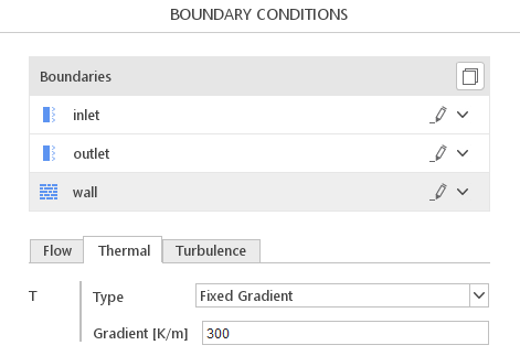
The definition of boundary conditions in SimFlow is both simple and intuitive. To specify the Fixed Gradient boundary condition, the user must navigate to the Boundary Conditions panel, select the appropriate boundary, and choose the correct option from the drop-down menu.
Fixed Gradient - SimFlow (OpenFOAM) Fixed Gradient - Alternatives
In this section, we propose boundary conditions that are alternative to Fixed Gradient. While they may fulfill similar purposes, they might be better suited for a specific application and provide a better approximation of physical world conditions.
| Boundary Condition | Description |
|---|---|
a very similar definition to Fixed Gradient but the prescribed normal gradient is set to zero | |
fixed value on a patch | |
convective heat transfer boundary condition that uses the Newton’s law of cooling | |
fixes the constant power expressed in \([W]\) | |
provides the heat flux directly |