Fixed Value - SimFlow (OpenFOAM) Description
Fixed Value is a boundary condition that specifies a constant value at a domain boundary and is one of the fundamental boundary conditions available in SimFlow (and OpenFOAM).
It is also referred to as the Dirichlet or First-Type boundary condition.
- \(\phi\) represents the solution variable (such as temperature or velocity)
- \(\phi_{0}\) denotes the constant value assigned to the boundary of the computational domain
Fixed Value can be applied to both scalar and vector fields, such as pressure, velocity, temperature, and others.
Fixed Value - SimFlow (OpenFOAM) Understanding Fixed Value
When the Fixed Value is applied, it enforces a specified value at the boundary. This value is uniformly applied to all mesh faces on the boundary, ensuring that it remains constant in time. In other words, the initially specified field, such as temperature or velocity, will not change during the simulation.
Fixed Value - Graphical Representation
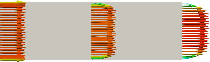
The image depicts a 2D computational fluid dynamics simulation domain. In this example, the boundary condition on the left boundary patch is set to a constant velocity of 1 m/s along the channel’s axis. As the flow field develops within the domain along the flow direction, the value changes near the wall but remains constant at the entrance boundary.
It is worth noting that on the border we can define not only a single constant value, but also a profile that varies along the boundary. The Fixed Value ensures that the specified value or profile remains unchanged throughout the simulation.
Fixed Value - Transient Simulation
The above animation demonstrates the Fixed Value used in a transient simulation. The left and right domain boundaries are at fixed temperatures set to 300K and 400K, respectively, while the bottom and top boundaries are insulated. The temperature profile maintains the fixed temperatures at the sides as time progresses.
Inlet Flux
The generic inlet flux \(J\) is the sum of diffusive and advective flux:
Fick’s law typically describes the diffusive flux and the total inlet flux can be described as:
where \(D\) is the diffusion coefficient and \(\phi\) is the transported scalar.
This equation implicates the interesting consequence. When the Fixed Gradient boundary condition is applied, only the diffusive part is controlled, but not the advective flux. Hence, the total flux will not be equal to the prescribed fixed gradient. The same applies when Fixed Value is used. In such a case, the advective flux will be defined but not the diffusive one.
In case of typical heat transfer problem, when Fixed Gradient is applied to the wall, the advective flux disappears (zero velocity at the wall) and the prescribed fixed gradient on the wall is proportional to the total heat flux. This, however, is not true when we have an inlet into the domain, with a specified velocity. It is important to understand that the total flux includes advective and diffusive terms. Misunderstanding might appear for so-called convective inlet boundary condition.
Convective Inlet
Let’s assume that we want to prescribe velocity and a scalar value \(\phi\) (for example, gas component concentration) at the inlet. Assuming a steady state solution, we would expect to get the same total mass flux associated with the given gas component exiting the domain. However, it is important to remember that the total flux takes the advective and diffusive components:
Therefore, the diffusive flux might also increase the concentration entering the fluid domain. The effect of increased concentration will be even higher with decreasing velocity at the inlet. As long as the inlet velocity is significant, the diffusive flux can be neglected, because inlet values quickly reach the first cell, making the gradient very low and convective flux dominates.
Fixed Value - SimFlow (OpenFOAM) Application & Physical Interpretation
The Fixed Value is one of the most commonly used boundary conditions. It consistently fixes the value of a specific variable at the domain boundary. However, its physical meaning varies depending on the problem being considered and the solver applied. Below are a few examples demonstrating how this boundary condition can be used and how to correctly interpret its meaning.
Fixed Value in Aerodynamics applications
Example applications: car, aircraft aerodynamics, wind tunnel experiment
These types of simulations can be solved using the simpleFoam (solver) This solver has two basic independent variables: pressure and velocity. Additionally, turbulence-related variables can be defined. The Fixed Value can be applied to the domain inlet to represent a constant inlet velocity. It can also be applied to the domain outlet to simulate a constant pressure outflow, such as atmospheric pressure.
| Physics | Pressure | Velocity |
|---|---|---|
Velocity Inlet | Zero Gradient | Fixed Value |
Pressure Outlet | Fixed Value | Zero Gradient |
| Tutorial | Description |
|---|---|
Excellent introductory tutorial to SimFlow, where the fundamental aspects of the software are given. The tutorial focuses on the water flow through a simple T-pipe geometry. | |
External aerodynamic analysis based on the car example. The simulation case includes symmetry conditions and turbulence modeling. |
Fixed Value in VoF (Volume of Fluid) applications
Example applications: free surface flows, ship hull calculations, sloshing, ship hydrodynamics, wave impact on structures
Problems that require resolving the sharp interface between two fluids, such as water and air, can be calculated using the interFoam (solver) The phase fraction, represented by \(\alpha\), differentiates between the fluids. The Fixed Value is typically used to define the fixed level of the first phase at the entry to the domain. For example, this boundary condition can be employed to set the constant water level in a pipe inlet.
| Physics | Pressure | Velocity | Phases \(\alpha\) |
|---|---|---|---|
Water Inlet | Zero Gradient | Fixed Value | Fixed Value |
| Tutorial | Description |
|---|---|
Simulation of a ship hull floating on a water surface in a two-phase flow (water and air) using Dynamic Mesh functionality with constraints. |
Fixed Value in Heat Transfer applications
Example applications: room ventilation, room heating, electronic cooling, atmospheric flows
The Fixed Value defines the temperature at a given boundary. This may represent, for example, the temperature of a hot radiator or the inlet temperature of air in a ventilation system.
| Physics | Pressure | Velocity | Thermal T |
|---|---|---|---|
Air Inlet | Fixed Flux Pressure | Surface Normal Fixed Value | Fixed Value |
| Tutorial | Description |
|---|---|
Cooling a steel cylinder with water, using a simplified 2D multi-region mesh to solve a conjugate heat transfer problem and track temperature fields over time. |
Fixed Value in Species Transport applications
Example applications: industrial furnaces, jet engines, chemical process industry (chemically reacting foams)
The reactingFoam (solver) can be applied for chemically reacting flows that involve heat transfer and chemical reactions with the combustion. In this application, the Fixed Value defines, for example, the constant gas composition at a given boundary.
| Physics | Pressure | Velocity | Species |
|---|---|---|---|
Air Inlet | Zero Gradient | Free Stream Velocity | Fixed Value |
Fixed Value - SimFlow (OpenFOAM) Fixed Value in SimFlow
The Fixed Value boundary condition can represent a different type of data: scalar and vector.
The Fixed Value allows not only prescribing a single value, but also a function of x, y, and z coordinates \(f=f(x,y,z)\). For example, a parabolic velocity profile can be prescribed, which will be constant in time (on the boundary) but will vary on the inlet patch depending on x, y and z coordinates.
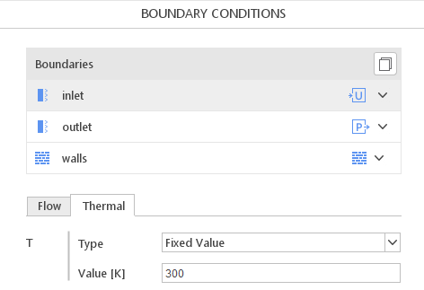
Fixed Value as a Scalar in SimFlow
When a scalar value is defined, such as pressure or temperature, only a single value needs to be specified. In the example below, a constant temperature is set at the inlet of the domain.
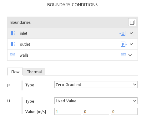
Fixed Value as a Vector in SimFlow
In the case of a vector field, the user must specify three components in the major directions: x, y, and z. Example below illustrates how the Fixed Value is applied to the inlet boundary.
Fixed Value - Value Patch
The Fixed Value is a primitive boundary condition, that effectively applies a solution value to the domain boundary, and later on this value is maintained throughout the simulation. However, since it directly imposes the solution and maintains it throughout the simulation, users might take advantage of the initial condition patching to overwrite values in a specified boundary region.
This feature can be used, for example, to define non-uniform concentration at the inlet, where the user wants to have a non-zero concentration only in the center of the inlet patch and a zero concentration on the rest of the patch. In such a scenario, we would define the Fixed Value with concentration equal to 0, and then patch only the center of the inlet patch (marked using a geometry) with the desired concentration value.
The patching operation is available in Patch Initialization.
Fixed Value - SimFlow (OpenFOAM) Fixed Value - Alternatives
In this section, we propose boundary conditions that are alternative to Fixed Value. While they may fulfill similar purposes, they might be better suited for a specific application and provide a better approximation of physical world conditions.
| Boundary Condition | Description |
|---|---|
uniform value on the patch, which vary over time | |
condition provides surface-normal vector boundary condition |