Jayatilleke Wall Function - SimFlow (OpenFOAM) Description
Jayatilleke Wall Function is a specialized wall-function boundary condition applied to the turbulent thermal diffusivity field \(\alpha_t\). It is typically used in conjunction with RANS-type turbulence models to improve near-wall prediction of heat transfer. The boundary condition leverages the Jayatilleke correlation, which provides a more accurate representation of the dimensionless temperature distribution in the near-wall region compared to simpler, more generic wall functions.
Jayatilleke Wall Function is typically used for:
- high-Reynolds number turbulent flows when the computational mesh does not fully resolve the viscous sublayer
- conjugate heat transfer and non-isothermal flows
- improved near-wall heat flux predictions - when standard wall functions do not guarantee sufficient accuracy
Jayatilleke Wall Function - SimFlow (OpenFOAM) Understanding Jayatilleke Wall Function
Jayatilleke Wall Function imposes a boundary condition on \(\alpha_t\) (the turbulent thermal diffusivity) at the wall that is consistent with the underlying physics and the turbulence model’s assumptions. Similarly to the momentum (viscous) wall functions, we can describe the non-dimensional temperature \(T^{*}\) (equivalent to the concept of non-dimensional velocity \(u^{*}\) as follows:
- \(T^{*}\) = \(Pr \cdot y^{*}\) for \(y^{*} < 5\)
- \(T^{*}\) = \(Pr_t \cdot (\frac{1}{\kappa}ln(E \cdot y^{*}) + P)\) for \(y^{*} > 30\)
- \(Pr\) - molecular (or laminar) Prandtl number
- \(Pr_t\) - turbulent Prandtl number
- \(P\) - term with strong dependence on Prandtl number
The equations above describe thermal viscous sublayer where conduction is important (for \(y^{*} < 5\)) and logarithmic law for the turbulent region where turbulence dominates over conduction (for \(y^{*} > 5\)).
When using thermal wall functions, we are interested in computing the thermal diffusivity used to approximate the wall heat transfer \(q_w\):
\(q_w = -k \frac{\partial T}{\partial y} = \rho c \alpha \frac{\partial T}{\partial y} = \rho c \alpha \frac{T_w - T_p}{y_p - y_w}\)
- \(T_w\) - temperature at the wall
- \(T_P\) - temperature at the cell center
- \(k\) - thermal conductivity
- \(\rho\) - density
- \(c_p\) - specific heat
- \(\alpha\) - thermal diffusivity
The thermal diffusivity coefficient \(\alpha_t\) is computed as follows:
- \(\alpha_t = \alpha \quad\) for \(\quad y^{*} < y_l^{*}\)
- \(\alpha_t = \frac{u_{\tau} y_p}{Pr_t (\frac{1}{\kappa} \ln(E \cdot y^{*}) + P)} \quad\) for \(\quad y^{*} > y_l^{*}\)
- \(y_l^*\) - the intersection between viscous and sub-region.
The relation for P is given by Jayatilleke function:
\(P = 9.24 ((\frac{Pr}{Pr_t})^{\frac{3}{4}} -1)(1+0.28e^{-0.007 \frac{Pr}{Pr_t}})\)
The final algorithm to compute the wall heat flux \(q_w\) is as follows:
- Compute \(y^{*}\)
- Compute Prandtl number \(Pr = \frac{\nu}{\alpha}\)
- Compute the intersection point \(y_l^{*}\)
- Compute the thermal diffusivity at the wall \(\alpha_w\)
- Compute the heat flux at the wall \(q_w\)
Jayatilleke Wall Function - SimFlow (OpenFOAM) Application & Physical Interpretation
Jayatilleke Wall Function is a specialized boundary condition for the turbulent thermal diffusivity \(\alpha_w\) at walls. It is used in RANS-type simulations when the wall-adjacent cells are not fully resolving the near-wall thermal boundary layer, and a wall-function approach is needed.
Jayatilleke Wall Function refines how the turbulent thermal diffusivity is modeled close to the wall. Instead of assuming a uniform turbulent Prandtl number, it uses empirical correlations (Jayatilleke’s function) that reflect how turbulence affects heat transfer. By doing so, it ensures that the temperature distribution near the wall more closely represents actual physical behavior, leading to improved predictions of wall heat flux and overall thermal performance.
Jayatilleke Wall Function in HVAC applications
Example applications: non-isothermal flows like HVAC ducts, thermal comfort
These types of simulations can be solved using the buoyantSimpleFoam (solver). In calculations with heat transfer it is necessary to correctly predict the temperature distribution which affects for example the thermal comfort of the people in a closed space.
| Physics | Pressure | Velocity | T | \(\alpha_t\) |
|---|---|---|---|---|
Wall | Fixed Flux Pressure | No-Slip | Fixed Value | Jayatilleke Wall Function |
Jayatilleke Wall Function - SimFlow (OpenFOAM) Jayatilleke Wall Function in SimFlow
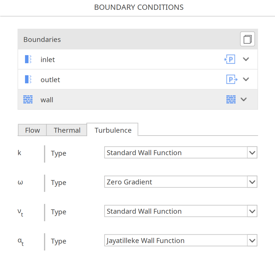
To define Jayatilleke Wall Function, the proper option must be selected from the drop-down menu for the turbulence field - Figure 1. No further input is required.
Jayatilleke Wall Function - SimFlow (OpenFOAM) Jayatilleke Wall Function - Alternatives
In this section, we propose boundary conditions that are alternative to Jayatilleke Wall Function. While they may fulfill similar purposes, they might be better suited for a specific application and provide a better approximation of physical world conditions.
| Boundary Condition | Description |
|---|---|
provides a wall function for turbulent viscosity (nut) |