Porous Baffle - SimFlow (OpenFOAM) Description
Porous Baffle is a boundary condition that introduces a pressure jump across a cyclic patch to model flow resistance through porous media. It is commonly used to simulate screens, filters, or baffles that impede flow without fully blocking it. It can be applied only to cyclic patches, allowing the simulation of flow through porous interfaces with additional drag effects.
Porous Baffle - SimFlow (OpenFOAM) Understanding Porous Baffle
Mathematically, the Porous Baffle boundary condition imposes a pressure jump across a cyclic patch to model flow resistance through porous media. It is expressed as:
- \(\Delta p\) – pressure drop across the porous interface \([Pa]\)
- \(D\) – Darcy coefficient \([\frac{1}{m^2}]\)
- \(\mu\) – dynamic viscosity \([Pa\cdot s]\)
- \(U\) – velocity normal to the patch \([\frac{m}{s}]\)
- \(I\) – inertial coefficient \([\frac{1}{m}]\)
- \(\rho\) – fluid density \([\frac{kg}{m^3}]\)
- \(L\) – thickness of the porous medium \([m]\)
This formulation combines viscous and inertial resistance terms, similar to the Forchheimer equation used in porous media modeling. The Darcy term dominates at low velocities, while the inertial term becomes significant at higher flow rates.
Assumptions and Limitations
- Time dependence: D and I can be time-dependent entries, so the boundary condition updates coefficients each timestep from the function evaluation.
- Cyclic patch requirement: The boundary condition only works on cyclic patches, meaning it cannot be used on arbitrary boundaries.
- Normal velocity assumption: The pressure drop is computed using the velocity normal to the patch. Complex flow patterns with significant tangential components may not be accurately represented.
- Single-phase incompressible flow: The formulation assumes a single-phase fluid with constant or slowly varying density. Compressibility effects are not accounted for.
- No turbulence modeling: The pressure drop is purely based on laminar viscosity and inertial resistance. Turbulent effects within the porous medium are not modeled.
- No temperature coupling: The resistance coefficients are independent of temperature, which may limit accuracy in thermally sensitive flows.
These limitations mean that while Porous Baffle is powerful for modeling screens and baffles, it should be used with care in multi-physics or high-speed applications.
The accuracy of the boundary condition depends heavily on the correct specification of the Darcy and inertial resistance coefficients. These coefficients control how much pressure drop is imposed across the porous interface and must reflect the physical characteristics of the screen, mesh, or baffle being modeled.
Understanding the Coefficients
- Darcy coefficient \(D\) \([1/m^2]\) – represents viscous resistance. Dominates at low velocities. Related to permeability \(K\) by \(D = \mu / K\).
- Inertial coefficient \(I\) \([1/m]\) – represents form drag and inertial losses. Becomes significant at higher velocities or with coarse, bluff structures.
- Length \(L\) \([m]\) – physical thickness of the porous medium. Used to scale the pressure drop.
The total pressure drop is computed as:
This equation mirrors the Forchheimer model used in porous media flow.
How to Choose D and I
There are three common approaches to tuning:
- Empirical Data: Use manufacturer data or experimental measurements of pressure drop vs. velocity. Fit the data to the Forchheimer equation to extract D and I.
- Analytical Estimation: For screens or perforated plates, use correlations from fluid mechanics literature. For example: for a wire mesh \(D = \frac{150 (1 - \epsilon)^2}{\epsilon^3 d_p^2}\), \(I = \frac{1.75 (1 - \epsilon)}{\epsilon^3 d_p}\), where \(\epsilon\) is porosity and \(d_p\) is pore diameter.
- Calibration: Run a simplified simulation with known flow and pressure drop, then adjust D and I until the simulated pressure loss matches the expected value.
Porous Baffle - SimFlow (OpenFOAM) Application & Physical Interpretation
The Porous Baffle boundary condition is designed to impose a pressure drop across a cyclic patch, simulating the resistance caused by porous media such as screens, filters, or baffles. It is particularly useful in single-phase incompressible flow simulations where localized flow resistance must be modeled without introducing volumetric source terms. Its physical interpretation depends on the flow regime and the geometry of the porous interface, especially in cases involving rotating machinery, HVAC systems, or industrial separators.
Porous Baffle in Rotating Machinery and Turbomachinery Applications
Example applications: fans, compressors, turbines, swirl generators.
These simulations are often solved using the simpleFoam (solver) or pisoFoam (solver), which handle steady or transient incompressible flows. The Porous Baffle boundary condition can be applied across cyclic patches separating rotating and stationary domains, where a screen or baffle introduces a known pressure loss. It enables accurate modeling of flow resistance without requiring detailed meshing of the porous structure.
Physics | Pressure | Velocity |
Cyclic Interface with Baffle | Porous Baffle | Cyclic |
Inlet | Fixed Value | Fixed Value |
Outlet | Zero Gradient | Zero Gradient |
Porous Baffle in HVAC and Process Engineering Applications
Example applications: duct systems, industrial filters, chemical separators.
These types of simulations may use the buoyantSimpleFoam (solver), which models buoyant incompressible flows. The Porous Baffle boundary condition can be applied at internal cyclic boundaries to represent flow resistance through porous partitions or mesh screens. This helps maintain realistic pressure gradients and avoids artificial acceleration or deceleration of flow through unresolved geometry.
Physics | Pressure | Velocity |
Porous Screen | Porous Baffle | Cyclic |
Air Supply Inlet | Fixed Value | Fixed Value |
Exhaust Outlet | Zero Gradient | Zero Gradient |
Porous Baffle - SimFlow (OpenFOAM) Porous Baffle in SimFlow
The definition of boundary conditions in SimFlow is both simple and intuitive. To specify the Porous Baffle boundary condition, the user must navigate to the Boundary Conditions panel, select the appropriate boundary for the pressure (either \(p\) or \(p-\rho gh\)) , and choose the correct option from the drop-down menu Figure 1.
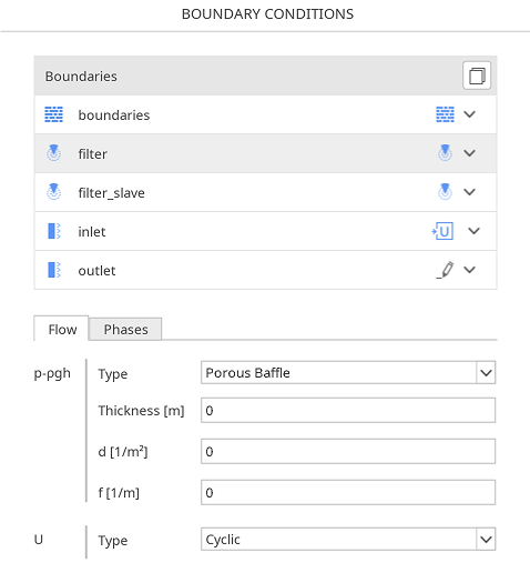
The following parameters need to be defined by the User:
Thickness - thickness of the porous baffle \([m ] \)
d - Darcy coefficient \([\frac{1}{m^2} ] \)
f - Inertial coefficient \([\frac{1}{m} ] \)
Porous Baffle - SimFlow (OpenFOAM) Porous Baffle - Alternatives
In this section, we propose boundary conditions that are alternative to Porous Baffle. While they may fulfill similar purposes, they might be better suited for a specific application and provide a better approximation of physical world conditions.
Boundary Condition | Description |
applies a user-defined jump in pressure or other fields across a cyclic patch, without computing it from flow resistance | |
enforces continuity across periodic boundaries, with no pressure drop or resistance | |
models pressure drop across a fan or porous interface using empirical or polynomial relations, suitable for HVAC and machinery |