Standard Wall Function - SimFlow (OpenFOAM) Description
Standard Wall Function is a boundary condition used for turbulent flow simulations, applicable to walls of the domain in the context of wall functions. Wall functions are an essential component in turbulence modeling, especially when using Reynolds-Averaged Navier-Stokes (RANS) models, as they bridge the solution between the fully turbulent region of the flow and the wall region, which is often not fully resolved in practical simulations due to computational constraints.
Standard Wall Function works like Zero Gradient, which can be used for the turbulent kinetic energy (i.e. k), square-root of turbulent kinetic energy (i.e. q), and Reynolds stress symmetric-tensor fields (i.e. R) for the cases of high Reynolds number flow using wall functions. The boundary condition assumes that turbulent quantities naturally adjust in this region, making it unnecessary to explicitly specify them by setting specific values. Unlike rough wall functions (e.g., nutkRoughWallFunction), this BC is for smooth walls and acts as a zero-gradient wrapper.
Standard Wall Function - SimFlow (OpenFOAM) Understanding Standard Wall Function
In channel flow, pipe flow, or flow around structures, the influence of the wall becomes more pronounced as the distance to the wall decreases. This is because the boundary layer develops along the wall, where viscous forces dominate and affect the velocity profile. Near the wall, the fluid experiences a no-slip condition, causing the velocity to drop to zero at the surface and creating a gradient in the velocity profile. As a result, the wall’s presence significantly impacts flow characteristics such as shear stress, turbulence, and pressure distribution.
In numerical simulations, there are two approaches for so-called near wall treatment:
- Direct Numerical Simulation (DNS) that resolves eddies in all scale but requires in return a very fine mesh and high computational power
- RANS and LES models, as they bridge the solution between the fully turbulent region of the flow and the wall region, which is often not fully resolved in practical simulations due to computational constraints.
Wall functions in computational fluid dynamics (CFD) are essential tools for modeling turbulent boundary layers in high Reynolds number flows. They provide a way to approximate the effects of the near-wall region, which can be computationally expensive to resolve directly due to the thinness of the viscous sublayer and the rapid changes in velocity and other flow properties.
Figure 1 represents the wall function profile with three characteristic regions: viscous sub-layer, buffer layer and log-law lawyer
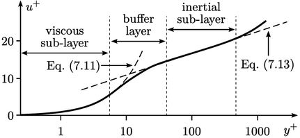
Wall functions bridge the gap between the wall and the first computational cell in a mesh. They are based on empirical correlations and theoretical considerations of the boundary layer structure. Here’s a breakdown of how wall functions interact with different regions of the boundary layer:
- Viscous Sublayer:
This is the region closest to the wall where viscous effects dominate and the flow is approximately laminar. The velocity profile in this region is linear with respect to the wall distance. In CFD models using wall functions, the viscous sublayer is not explicitly resolved. Instead, the wall functions account for its effects through empirical correlations.
- Buffer Region:
Located between the viscous sublayer and the log-law region, the buffer region is a transition area where both viscous and turbulent effects are significant. Wall functions typically do not model the buffer region explicitly but instead provide a smooth transition between the empirical expressions used for the viscous sublayer and the log-law region.
- Log-Law Region:
Further from the wall is the logarithmic region where turbulence effects dominate, and the velocity profile follows the logarithmic law of the wall. This region can be expressed as:
- \(U^+\) - the dimensionless velocity
- \(\kappa\) - the von Karman constant
- \(y^+\) - the dimensionless wall distance
- \(B\) - an empirical constant
Standard Wall Function is a wrapper around Zero Gradient because the turbulent quantities, such as turbulent kinetic energy \(k\), is often assumed to be nearly uniform. This assumption is valid due to the balance between production and dissipation of turbulence in this region. Standard Wall Function assumes that the turbulent quantities adjust themselves naturally in this region and that explicit specification (like setting a specific value) is unnecessary.
By using Zero Gradient, Standard Wall Function allows the wall shear stress and other related quantities to dictate the distribution of k in a manner consistent with the underlying turbulence model and wall function approach.
Standard Wall Function - SimFlow (OpenFOAM) Application & Physical Interpretation
The Standard Wall Function is a commonly used boundary condition in turbulent flows. It is primarily used in the context of wall functions for turbulent flow simulations, which are an essential component in turbulence modeling, especially when using Reynolds-Averaged Navier-Stokes (RANS) models, as they bridge the solution between the fully turbulent region of the flow and the wall region. Below are a few examples demonstrating how this boundary condition can be used and how to correctly interpret its meaning.
Standard Wall Function in Aerodynamics applications
Example applications: aircraft aerodynamics with compressibility
These types of simulations can be solved using the rhoSimpleFoam (solver). The Standard Wall Function can be applied to the wall boundary which represents the wing or the hull of the airplane.
| Physics | Pressure | Velocity | Temperature | k | \(\omega\) |
|---|---|---|---|---|---|
Wing | Zero Gradient | No-Slip | Zero Gradient | Standard Wall Function | Standard Wall Function |
Standard Wall Function in Channel Flow and Pipe Flow applications
Example applications: channel and pipe flow, T-junctions
These types of simulations can be solved using the simpleFoam (solver). The Standard Wall Function can be applied to the wall boundary which represents the channel flows
| Physics | Pressure | Velocity | k | \(\epsilon\) |
|---|---|---|---|---|
Channel | Zero Gradient | No-Slip | Standard Wall Function | Standard Wall Function |
Standard Wall Function - SimFlow (OpenFOAM) Standard Wall Function in SimFlow
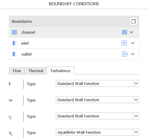
To define Standard Wall Function on the wall boundary, the proper option must be selected from the drop-down menu in the Turbulence tab - Figure 2. Please note that the Turbulence tab will be visible only if the turbulence equations are activated (Turbulence panel).
Standard Wall Function - SimFlow (OpenFOAM) Standard Wall Function - Alternatives
In this section, we propose boundary conditions that are alternative to Standard Wall Function. While they may fulfill similar purposes, they might be better suited for a specific application and provide a better approximation of physical world conditions.
| Boundary Condition | Description |
|---|---|
belongs to the Neumann boundary conditions, sets the normal gradient of any variable to zero | |
fixed value on the patch | |
works in a similar way to Standard Wall Function, but can mimic the surface roughness |