Standard Wall Function (k) - SimFlow (OpenFOAM) Description
Standard Wall Function (k) is a boundary condition that provides a wall function for the turbulent viscosity \(\nu_t\) based on the turbulent kinetic energy \(k\) for low- and high-Reynolds number applications. It inherits from the Dirichlet boundary condition (Fixed Value) and applies to walls of the numerical domain.
It is typically used with turbulence models like \(k-\epsilon\) or \(k-\omega\), particularly in cases where the flow is fully turbulent near the wall, and a wall function approach is preferred over resolving the boundary layer fully down to the wall. Standard Wall Function (k) is suited for situations where the mesh near the wall does not resolve the viscous sublayer (i.e., when the \(y^+\) value is not very small), making it necessary to apply a wall function to model the turbulence effects properly.
Wall functions are a crucial element in turbulence modeling, particularly with Reynolds-Averaged Navier-Stokes (RANS) models. They connect the solution between the fully turbulent flow region and the wall region, which is often not fully resolved in practical simulations due to computational limitations. Unlike nutkRoughWallFunction (rough walls) or nutURoughWallFunction (velocity-based), this BC is designed for smooth walls with k-based calculations.
Standard Wall Function (k) - SimFlow (OpenFOAM) Understanding Standard Wall Function (k)
The wall function Standard Wall Function (k) provides a turbulent viscosity \(\nu_t\) condition based on the turbulent kinetic energy \(k\) calculated according to:
with
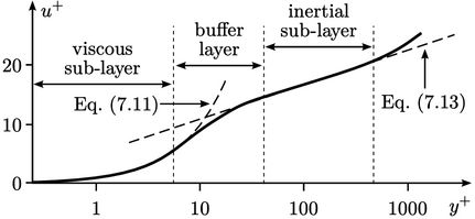
when \(y^+ < y_{lam}^+\)
- \(\nu_t\) - Turbulent Viscosity \([\frac{m^{2}}{s}]\)
- \(\nu_{t_{vis}}\) - \(\nu_t\) Computed by the Viscous Sublayer Assumptions \([\frac{m^{2}}{s}]\)
- \(\nu_{t_{log}}\) - \(\nu_t\) Computed by the Inertial Sublayer Assumptions \([\frac{m^{2}}{s}]\)
- \(\nu_w\) - Kinematic Viscosity of Fluid Near Wall \([\frac{m^{2}}{s}]\)
- \(y^+\) - Estimated Wall-Normal Height of the Cell Centre in Wall Units \(-\)
- \(\kappa\) - von Kármán Constant \(-\)
- \(E\) - Wall Roughness Parameter \(-\)
- \(C_\mu\) - Empirical Model Constant \(-\)
- \(y\) - Wall-Normal Height \([m]\)
- \(k\) - Turbulent Kinetic Energy \([\frac{m^{2}}{s^{2}}]\)
- \(f_{blend}\) - Wall-Function Blending Operator Between the Viscous and Inertial Sublayer Contributions
Standard Wall Function (k) - SimFlow (OpenFOAM) Application & Physical Interpretation
Standard Wall Function (k) is crucial for accurately simulating flows in ducts and pipes, but also external flows whenever the turbulent flows are considered, and wall presence affects the flow. Standard Wall Function (k) approximates the effect of the near-wall turbulence and does not require the mesh to resolve the viscous sublayer directly. Instead, it bridges the gap between the wall and the first computational cell by using an empirical relationship based on the turbulence model.
Standard Wall Function (k) in Pipe Flow applications
Example applications: pipe or duct flow
These types of simulations can be solved using the pimpleFoam (solver). In this case, we assume that the inner surface of the pipe is not perfectly smooth, but rather is characterized with some roughness.
| Physics | Pressure | Velocity | \(k\) | \(\epsilon\) | \(nu_t\) |
|---|---|---|---|---|---|
Pipe (Wall) | Zero Gradient | No-Slip | Standard Wall Function | Standard Wall Function | Standard Wall Function (k) |
Standard Wall Function (k) in Compressible Aerodynamics applications
Example applications: External Aerodynamics (Airfoils)
These types of simulations can be solved using the rhoSimpleFoam (solver).
| Physics | Pressure | Velocity | Temperature | \(k\) | \(\omega\) | \(\nu_t\) |
|---|---|---|---|---|---|---|
Airfoil(Wall) | Zero Gradient | No-Slip | Zero Gradient | Standard Wall Function | Standard Wall Function | Standard Wall Function (k) |
Standard Wall Function (k) in HVAC applications
Example applications: Room Heating
These types of simulations can be solved using the buoyantBoussinesqPimpleFoam (solver).
| Physics | Pressure | Modified Pressure \(p_rgh\) | Velocity | Temperature | \(k\) | \(\epsilon\) | \(nu_t\) |
|---|---|---|---|---|---|---|---|
Room walls (Wall) | Calculated | Fixed Flux Pressure | No-Slip | Fixed Value | Standard Wall Function | Standard Wall Function | Standard Wall Function (k) |
Standard Wall Function (k) - SimFlow (OpenFOAM) Standard Wall Function (k) in SimFlow
To define Standard Wall Function (k) on the wall boundary, the proper option must be selected from the drop-down menu in the Turbulence tab - Figure 1. Please note that the Turbulence tab will be visible only if the turbulence equations are activated (Turbulence panel).
Standard Wall Function (k) - SimFlow (OpenFOAM) Standard Wall Function (k) - Alternatives
In this section, we propose boundary conditions that are alternative to Standard Wall Function (k). While they may fulfill similar purposes, they might be better suited for a specific application and provide a better approximation of physical world conditions.
| Boundary Condition | Description |
|---|---|
fixed value on the patch | |
works in a similar way to Standard Wall Function (k), but can mimic the surface roughness |