Wave - SimFlow (OpenFOAM) Description
Wave is a boundary condition which prescribes the fluid velocity according to a chosen wave theory (e.g., Shallow Water Absorption, Stream Function, Boussinesq, Cnoidal, Stokes I, Stokes II and Stokes V) so that physical wave motions are introduced into the computational domain. This boundary condition is applicable for velocity and phase fraction fields, both inlet and outlet patches. It is commonly used in wave generation zones for free-surface flow simulations, particularly in coastal and offshore hydrodynamics.
Wave - SimFlow (OpenFOAM) Understanding Wave
Mathematically, the Wave boundary condition imposes a time- and space-dependent velocity field at a boundary using analytical wave theory. It is expressed as:
- \(\vec{U}(\vec{x}, t)\) – velocity vector at boundary face \([m/s]\)
- \(\vec{x}\) – spatial location on the patch \([m]\) \(t\) – simulation time [s],
\(\vec{U}_{wave}\) – wave-induced velocity from analytical wave theory [m/s].
This formulation prescribes the velocity field based on the instantaneous wave orbital motion, ensuring realistic wave inflow conditions in free-surface simulations.
Assumptions and Limitations:
- Prescribed motion only: The boundary condition does not account for reflected waves or feedback from the domain.
- Single wave model per patch: Only one wave theory can be active at a time.
- No viscous effects: Most wave models assume inviscid flow.
- Flat patch assumption: Accuracy may degrade on complex or curved boundaries.
- Coupling required: Wave must be also used for \(\alpha\) to ensure consistent phase fraction evolution.
Wave Theories in SimFlow
Several wave theories are supported by SimFlow. The wave model should be appropriate for the wave steepness, depth regime and nonlinearity of your case. Mismatch between model assumptions and physical regime will degrade accuracy.
Shallow Water Absorption (Shallow-water theory / nonlinear shallow-water)
The shallow water absorption model is based on depth-averaged shallow-water equations (Saint-Venant / nonlinear shallow-water). It links free-surface elevation \(\eta(x,t)\) and depth-averaged velocity \(u(x,t)\) through conservation of mass and momentum.
For linear long waves in shallow water:
- \(h\) is the local water depth \([m]\)
- \(A\) is the wave amplitude \([m]\)
- \(\omega\) is the angular frequency \([rad/s]\)
- \(k\) is the wavenumber \([1/m]\)
The dispersion relation for long waves is:
Assumptions:
- \(kh \ll 1\): wavelength much larger than depth,
- Vertical velocity structure is nearly uniform,
- Non-dispersive or weakly dispersive behavior.
Applications:
- Surf zones and coastal wave modeling,
- Tidal wave propagation,
- Large-scale harbor and flood simulations,
- Absorption boundary layers (non-reflecting shallow-water absorbers).
Limitations:
- Not valid for intermediate or deep water,
- Inaccurate for short wavelengths,
- Dispersion and vertical velocity variation are neglected.
Stream Function theory
The stream function wave theory models nonlinear periodic waves in finite depth using a spectral solution. The free-surface elevation is given by:
- \(h\) is the mean water depth \([m]\)
- \(E_j\) are Fourier coefficients
- \(k\) is the wavenumber \([1/m]\)
- \(\omega\) is the angular frequency \([rad/s]\)
- \(\phi\) is the phase shift \([rad]\)
This theory solves a nonlinear boundary-value problem for a stream function \(\Psi(x,z)\) that satisfies:
with nonlinear free-surface boundary conditions.
The solution is obtained iteratively using spectral or collocation methods. The surface elevation \(\eta\) and velocity components are derived from stream function gradients:
Assumptions:
- Nonlinear wave behavior,
- Finite water depth,
- Inviscid, irrotational flow,
- Valid for steep waves up to near-breaking conditions.
Applications:
- Accurate generation of highly nonlinear regular waves,
- Intermediate-depth wave flumes,
- Engineering wave-maker boundary conditions,
- Steep wave validation tests.
Limitations:
- Requires precomputed Fourier coefficients,
- Computationally intensive due to iterative solution,
- Sensitive to parameter choices,
- May struggle with breaking waves or strongly transient phenomena.
Boussinesq Waves
Boussinesq-type solitary waves are modeled using an analytical solution that balances nonlinearity and dispersion in shallow water. The free-surface elevation is given by:
- \(\eta(x,t)\) – the free-surface elevation \([m]\)
- \(H\) – the wave height \([m]\)
- \(h\) – the water depth \([m]\)
- \(c\) – the wave celerity \([m/s]\)
- \(x\) – the horizontal coordinate \([m]\)
- \(t\) – time \([s]\)
This equation describes a solitary wave that maintains its shape while propagating through shallow water.
Boussinesq-type models solve depth-averaged equations that include both nonlinear and dispersive terms. These models are ideal for simulating long waves in shallow water, especially solitary waves. The analytical solution is used to initialize the wave profile and velocity field in OpenFOAM, allowing the wave to propagate naturally.
Assumptions:
- \(kh \ll 1\): wavelength much larger than depth,
- Weak to moderate nonlinearity,
- Weak dispersion included,
- Depth-averaged flow (no vertical orbital structure),
- Inviscid and irrotational flow.
Applications:
- Solitary wave propagation.
- Tsunami modeling,
- Coastal and harbor wave studies,
- Benchmarking nonlinear wave interactions.
Limitations:
- Not suitable for deep water or short waves,
- Cannot represent vertical velocity profiles,
- Accuracy depends on grid resolution and dispersive term implementation,
- May not capture wave breaking or strong turbulence.
Cnoidal Waves
Cnoidal waves are nonlinear, periodic wave solutions suitable for shallow water. The free-surface elevation is given by:
- \(\eta(x,t)\) – the free-surface elevation \([m]\)
- \(h\) – the mean water depth \([m]\)
- \(E(m)\) – the complete elliptic integral of the second kind
- \(K(m)\) – the complete elliptic integral of the first kind
- \(\text{cn}\) – the Jacobi elliptic cosine function
- \(\lambda\) – the wavelength \([m]\)
- \(c\) – the wave celerity \([m/s]\) \(m\) – the elliptic modulus (0 < m < 1),
\(x\) – the horizontal coordinate [m],
\(t\) – time [s].
This formulation captures the nonlinear shape of long waves, with sharper crests and flatter troughs compared to sinusoidal waves.
Cnoidal waves are derived from the Korteweg–de Vries (KdV) equation and provide accurate representations of long, nonlinear waves in shallow water. The use of elliptic functions allows for precise control over wave steepness and shape. This analytical solution is used to initialize both the velocity and surface elevation fields for wave generation.
Assumptions:
- Shallow water: \(kh \ll 1\),
- Nonlinear wave behavior,
- Periodic wave train,
- Inviscid, irrotational flow.
Applications:
- Coastal and harbor wave modeling,
- Long wave propagation in shallow basins,
- Engineering design of breakwaters and wave flumes,
- Benchmarking nonlinear wave models.
Limitations:
- Not suitable for deep water or short waves,
- Requires evaluation of elliptic functions,
- Cannot represent breaking waves,
- Accuracy depends on elliptic modulus and wave parameters.
Stokes I Waves
Stokes I waves represent the simplest form of regular wave theory, suitable for small-amplitude waves in deep water. The free-surface elevation is given by:
- \(\eta(x,t)\) – the free-surface elevation \([m]\)
- \(H\) – the wave height \([m]\)
- \(k\) – the wavenumber \([1/m]\)
- \(\omega\) – the angular frequency \([rad/s]\)
- \(x\) – the horizontal coordinate \([m]\)
- \(t\) – time \([s]\)
The horizontal and vertical velocity components are derived from linear wave theory and vary with depth:
- \(u(x,z,t)\) – the horizontal velocity \([m/s]\)
- \(w(x,z,t)\) – the vertical velocity \([m/s]\)
- \(z\) – the vertical coordinate \([m]\)
- \(h\) – the water depth \([m]\)
Stokes I theory assumes linear wave behavior and is derived from the Airy wave solution. It is valid for small wave heights and deep water conditions. The velocity field exhibits a vertical orbital structure that decays exponentially with depth.
This model is used to initialize regular wave profiles and velocity fields for wave generation boundaries.
Assumptions:
- Small wave steepness: \(H/\lambda \ll 1\),
- Deep water: \(kh \gg 1\),
- Linear wave theory,
- Inviscid, irrotational flow.
Applications:
- Regular wave tanks,
- Offshore structure loading,
- Deep water wave propagation,
- Benchmarking linear wave models.
Limitations:
- Inaccurate for shallow water or steep waves,
- Cannot model nonlinear effects or wave breaking,
- Orbital motion decays rapidly with depth,
- Limited to sinusoidal wave shapes.
Stokes II Waves
Stokes II waves extend linear wave theory by including second-order nonlinear corrections, making them suitable for moderate wave steepness. The free-surface elevation is given by:
- \(\eta(x,t)\) – the free-surface elevation \([m]\)
- \(H\) – the wave height \([m]\)
- \(k\) – the wavenumber \([1/m]\)
- \(\omega\) – the angular frequency \([rad/s]\)
- \(\lambda\) – the wavelength \([m]\)
- \(x\) – the horizontal coordinate \([m]\)
- \(t\) – time \([s]\)
The second term introduces a harmonic component at twice the fundamental frequency, capturing the nonlinear wave shape with sharper crests and flatter troughs.
Stokes II theory improves upon linear (Stokes I) theory by incorporating second-order effects. This allows for more accurate modeling of wave asymmetry and steepness in intermediate-depth water. The velocity field also includes second-order corrections, enhancing the realism of orbital motion near the surface.
This model is used to initialize wave profiles and velocity fields for boundary conditions like waveVelocity and waveAlpha.
Assumptions:
- Moderate wave steepness: \(H/\lambda\) not too small,
- Deep or intermediate water: \(kh \gtrsim 1\),
- Inviscid, irrotational flow,
- Weak nonlinearity (second-order).
Applications:
- Offshore structure loading,
- Intermediate-depth wave tanks,
- Engineering wave-maker boundary conditions,
- Benchmarking nonlinear wave models.
Limitations:
- Less accurate for very steep or shallow waves,
- Cannot model wave breaking,
- Limited to periodic wave trains,
- Orbital motion still decays with depth.
Stokes V Waves
Stokes V waves are fifth-order approximations of nonlinear wave theory, suitable for steep waves in deep or intermediate water. The free-surface elevation is given by:
- \(\eta(x,t)\) – the free-surface elevation \([m]\)
- \(H\) – the wave height \([m]\)
- \(k\) – the wavenumber \([1/m]\)
- \(\omega\) – the angular frequency \([rad/s]\)
- \(\lambda\) – the wavelength \([m]\)
- \(x\) – the horizontal coordinate \([m]\)
- \(t\) – time \([s]\)
This fifth-order expansion captures multiple harmonics, allowing for accurate modeling of steep wave profiles with sharp crests and flat troughs.
Stokes V theory builds on lower-order Stokes approximations by including up to five harmonics in the wave profile. This allows for precise representation of nonlinear wave shapes and orbital velocities in deep or intermediate water. The velocity field also includes fifth-order corrections, making it suitable for engineering applications involving steep waves.
This model is used to initialize wave profiles and velocity fields for boundary conditions.
Assumptions:
- Moderate to steep wave steepness,
- Deep or intermediate water: \(kh \gtrsim 1\),
- Inviscid, irrotational flow,
- Periodic wave train,
- Valid for regular waves with high nonlinearity.
Applications:
- Offshore structure loading,
- Deep water wave tanks,
- Engineering wave-maker boundary conditions,
- Benchmarking nonlinear wave models.
Limitations:
- Not suitable for shallow water,
- Cannot model wave breaking,
- Computationally more intensive than lower-order models,
- Limited to periodic wave shapes.
Summary of Available Wave Models
| Wave Theory | Equation Type | Assumptions | Applications | Limitations |
|---|---|---|---|---|
Stokes I, II, V | Trigonometric series | Small to moderate steepness, deep water | Regular wave tanks, offshore structures | Inaccurate for shallow or steep waves |
Cnoidal | Elliptic functions (Jacobi cn) | Long waves, shallow water | Coastal engineering, harbor resonance | Complex math, not for deep water |
Stream Function | Fourier series with nonlinear corrections | Finite-depth, nonlinear | Steep wave modeling, wave flumes | Requires precomputed coefficients |
Boussinesq | Depth-averaged PDEs with dispersion | Weak nonlinearity, shallow water | Tsunami modeling, long wave propagation | Not valid for short or steep waves |
Shallow Water Absorption | Damping function based on depth and velocity | Outgoing wave absorption | Open boundaries, wave tanks | Not a wave generation model |
Wave - SimFlow (OpenFOAM) Application & Physical Interpretation
Wave boundary condition is designed to impose a time-dependent velocity field at the boundary, based on analytical wave theory.
It is particularly useful in free-surface simulations where wave generation is required at inflow boundaries.
Its physical interpretation depends on the selected wave model and the solver configuration, especially in cases involving regular, solitary, or shallow-water waves.
Wave in Coastal and Hydraulic Applications
Example applications: wave flumes, coastal structures, harbor resonance, beach erosion studies
These simulations are often solved using the interFoam (solver), which handles multiphase flows with a free surface.
The Wave boundary condition can be applied at inlet boundaries to generate realistic wave motion using theories such as Stokes, Cnoidal, or Boussinesq.
It ensures physically accurate wave kinematics without requiring manual specification of velocity profiles.
Example Boundary Conditions set for Hydraulic Wave Applications
Physics | Pressure | Velocity |
Zero Gradient | Wave | Wave Outlet |
phaseHydrostaticPressure | Zero Gradient | Atmospheric Opening |
Wave in Offshore and Structural Engineering Simulations
Example applications: offshore platform loading, wave impact studies, floating body dynamics
These types of simulations may use the interFoam (solver) or coupled solvers with dynamic mesh motion.
The Wave boundary condition can be applied at inflow boundaries to impose wave-induced orbital velocities, capturing both horizontal and vertical components.
This helps simulate realistic wave-structure interactions and supports validation against experimental wave tank data.
| Physics | Pressure | Velocity |
|---|---|---|
Wave Inlet | Zero Gradient | {waveVelocity} |
Solid Wall | Zero Gradient | No Slip |
Free Surface | Atmospheric | Zero Gradient |
Wave - SimFlow (OpenFOAM) Wave in SimFlow
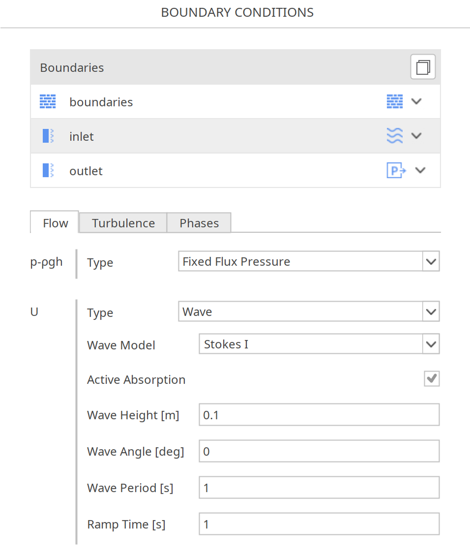
In SimFlow, the Wave boundary condition is applied to velocity (U) and phase fraction (alpha) fields at inlet boundaries for wave generation. Select "Wave" for both U and alpha from the boundary conditions panel. For velocity (U), choose the wave theory first (e.g., Stokes, Cnoidal), then specify wave parameters such as height, period, depth, and direction. For phase fraction (alpha), no additional parameters are required. This ensures accurate wave inflow for coastal or offshore simulations.
Wave - SimFlow (OpenFOAM) Wave - Alternatives
In this section, we propose boundary conditions that are alternative to Wave. While they may fulfill similar purposes, they might be better suited for a specific application and provide a better approximation of physical world conditions.
| Boundary Condition | Description |
|---|---|
imposes a constant velocity vector at the boundary, suitable for steady inflow but lacks wave dynamics | |
prescribes a velocity field that changes over time using tabulated input, useful for replaying measured wave data | |
allows velocity to be extrapolated from the interior, typically used at outflow or passive boundaries | |
switches between fixed value and zero gradient based on flow direction, useful for recirculating or open domains |