Discrete Phase
Introduction
The Discrete Phase panel defines models used for Lagrangian particle tracking approach.
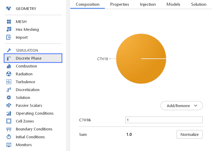
Composition
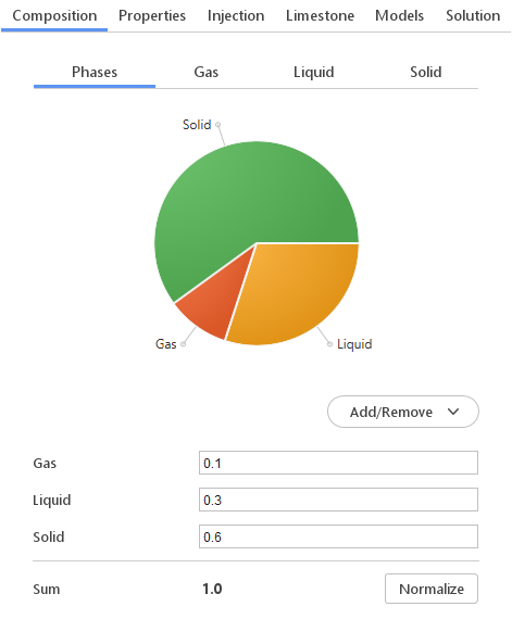
In the simulation that uses species transport model, the composition of the discrete phase have to be defined. If the discrete phase is liquid (e.g. spray droplets) one needs to specify which liquid compose the phase. If the discrete phase consists of multiple phases (e.g. coal particles), one needs to define composition in terms of each individual phase (gas, liquid, solid).
Adding/Removing Components
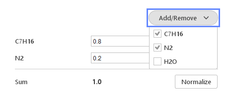
Add/Remove button shows the list of currently available components. By selecting the components from the drop-down menu, a given constituent is added to the edition list. Analogically, when a given component is deselected, it is removed from the edition list.
Editing Concentration
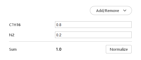
The concentration of each component can be specified next to the name of constituent.
You can specify the concentration of each of the component using the inputs on the right-hand side. The sum of concentrations does not have to be equal to 1. However if the sum is not equal to 1, the Sum will be displayed in red. You can always normalize the concentrations by clicking the Normalize button.
Properties
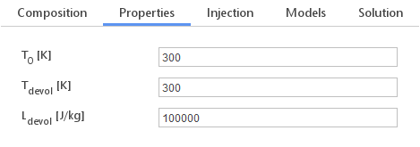
In the Properties tab, you can define material properties of the discrete phase. The inputs you need to specify may change depending on the currently selected solver.
Possible inputs:
- \(T_0 [K]\) - initial temperature
- \(\rho_0 [kg/m^3]\) - initial density
- \(T_{devol} [K]\) - devolatilization temperature
- \(L_{devol} [J/kg]\) - latent heat of devolatilization
- \(T_{limestone} [K]\) - limestone temperature
- \(E [Pa]\) - Young’s modulus
- \(\nu [-]\) - Poisson’s ratio
- \(e [-]\) - restitution coefficient
- \(\alpha_{packed} [-]\) - packed volume fraction
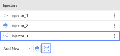
Injections
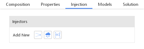
In the Injections tab, you can define injectors. An injector defines how particles are introduced into the domain. Currently, there are three types of injectors available:
- Cone Injector
- Boundary Injector
- Manual Injector
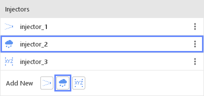
Injectors are created and manipulated using a standard list.
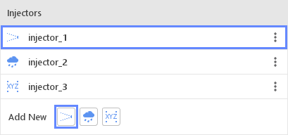
Editing Injectors
By selecting a given injector type in the Injectors list, properties will be displayed below it. Injector properties depend on the injector type. However, each injector will require specifying particle size distribution.
Cone Injector
The Cone injector can be used to represent an injection from a nozzle.
Cone Injection
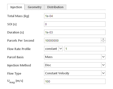
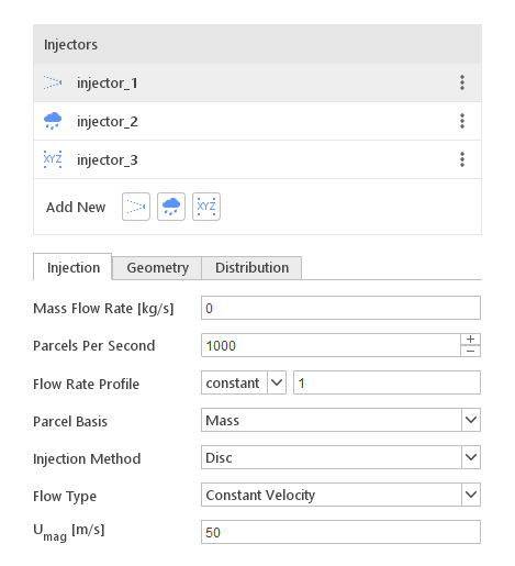
The Injection tab contain settings that define basic properties of the injector.
Inputs:
- Total Mass [kg] - total mass injected (available in transient simulations)
- SOI [s] - start of the injection (available in transient simulations)
- Duration [s] - duration of the injection (available in transient simulations)
- Mass Flow Rate [kg/s] - injection mass flow rate (available in steady-state simulations)
- Parcels Per Second - number of particles injected per second of the simulation
- Flow Rate Profile - flow rate profile relative to SOI
- Parcel Basis - input defines how number of particles per parcel are calculated
- Injection Method - input defines injector geometry type
- Flow Type - input defines how the velocity of particles is calculated
- \(\mathbf{U_{mag}} [m/s]\) - particle velocity
Cone Geometry
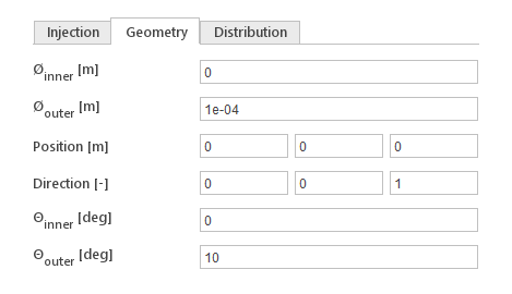
The Geometry tab defines the geometry of the cone.
Inputs:
- \(\phi_{inner} [m]\) - inner diameter of the inlet cone
- \(\phi_{outer} [m]\) - outer diameter of the inlet cone
- \(Position [m\)] - location of the inlet
- \(Direction [-\)] - direction of the inlet
- \(\theta_{inner} [deg]\) - inner angle of the cone
- \(\theta_{outer} [deg]\) - outer angle of the cone
Boundary Injector
The Boundary injector introduces particles into the domain through a boundary.
Boundary Injection
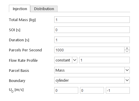
The Injection tab contain settings that define basic properties of the injector.
Inputs:
- Total Mass [kg] - total mass injected (available in transient simulations)
- SOI [s] - start of the injection (available in transient simulations)
- Duration [s] - duration of the injection (available in transient simulations)
- Mass Flow Rate [kg/s] - ijection mass flow rate (available in steady-state simulations)
- Parcels Per Second - number of particles injected per second of the simulation
- Flow Rate Profile - flow rate profile relative to SOI
- Parcel Basis - input defines how number of particles per parcel are calculated
- Boundary - boundary from which the particles will be introduced
- \(\mathbf{U_0} [m/s]\) - initial particle velocity
Manual Injector
The Manual injector introduces particles into the domain at specific locations. All the particles are introduced at the start of injection.
Manual Injection
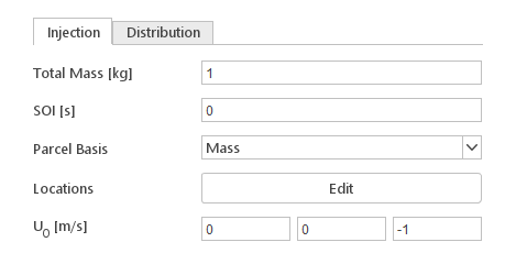
The Injection tab contain settings that define basic properties of the injector.
Inputs:
- Total Mass [kg] - total mass injected
- SOI [s] - moment of the injection
- Parcel Basis - input defines how number of particles per parcel are calculated
- Locations - coordinates of injection points
- \(\mathbf{U_0} [m/s]\) - initial particle velocity
Particle Size Distribution
In the Distribution tab of the injector the diameter distribution of the particles introduced by the injector is defined. Currently, available distribution models:
- Fixed
- Uniform
- Rosin-Rammler
- Normal
- Exponential
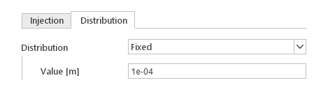
Fixed Distribution
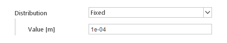
The Fixed distribution model fixes diameters of all particles to a specified value.
Inputs:
- Value [m] - fixed diameter
Uniform Distribution
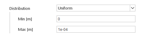
With the Uniform distribution particle diameters have a uniform probability to be in a specified range.
Inputs:
- Min [m] - mimimal allowed diameter
- Max [m] - maximal allowed diameter
Rosin-Ramler Distribution
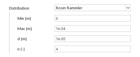
With the Rosin-Ramler distribution, particle diameters have probability calculated from the Rosin-Rammler formula.
Inputs:
- Min [m] - mimimal allowed diameter
- Max [m] - maximal allowed diameter
- d [m] - most probable diameter
- n [-] - distribution parameter
Normal Distribution
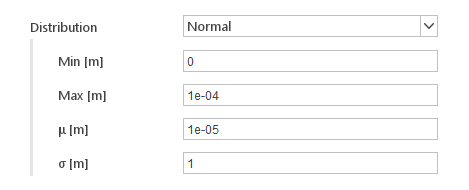
With the Normal distribution particle, diameters have probability calculated from the normal distribution .
Inputs:
- Min [m] - minimal allowed diameter
- Max [m] - maximal allowed diameter
- \(\mu [m\)] - mean diameter
- \(\sigma [m]\) - standard deviation
Exponential Distribution
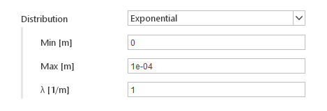
With the Exponential distribution, particle diameters have probability calculated using the exponential function.
Inputs:
- Min [m] - minimal allowed diameter
- Max [m] - maximal allowed diameter
- \(\lambda [1/m]\) - exponent coefficient
Limestone Injectors
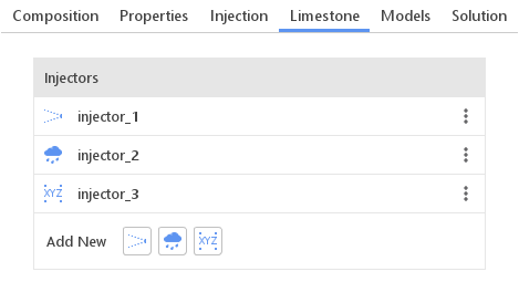
The Limestone tab is available for Coal Chemistry solver. Here one can define limestone injectors. Similarly to the typical injectors, there are three types available:
- Cone Injector
- Boundary Injector
- Manual Injector
Injectors are created and manipulated using a standard list.
Models
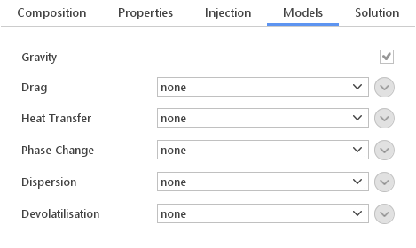
In the Models tab one can enable various models that should influence the behavior of the particles. Models available in this tab depend on the selected solver.
Gravity

The Gravity input defines whether particles should be the subject to the force of gravity.
Drag Models

These models define how drag forces are calculated when a particle moves relative to the fluid. Available drag models:
- Sphere Drag - model assumes that each particle is a solid sphere
- Ergun-Wen-Yu - Ergun-Wen-Yu model for dense particle clouds
- Wen-Yu - Wen-Yu model for dense particle clouds
- Plessis-Masliyah - Plessis-Masliyah model for dense particle clouds
Models available for selection are dependent on the currently selected solver.
Heat Transfer Models
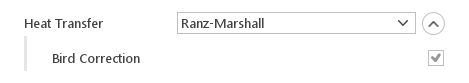
These models define how heat is transferred between particles and the fluid. Available models:
- Ranz-Marshall - uses Ranz-Marshall correlation with optional Bird Correction
Phase Change Models
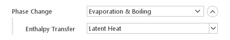
These models define how mass from particles is introduced into the continuous phase. Available phase change models:
- Evaporation - liquid in particles is converted to gas through evaporation
- Evaporation & Boiling - liquid in particles is converted to gas through evaporation and boiling
For each of the phase change models, the way enthalpy is transferred to the continuous phase must be specified. Available Enthalpy Transfer models:
- Latent Heat - uses only latent heat
- Enthalpy Difference - uses the difference between gas enthalpy and latent heat
Dispersion Models
These models introduce dispersion of particles due to turbulence. Available dispersion models:
- Stochastic - the velocity of particles is perturbed in random direction
- Gradient - the velocity of particles is perturbed in the opposite direction of the turbulent kinetic energy gradient
Devolatilisation Models
These models define how gaseous components of the particle are introduced into the continuous phase. Available devolatilization models:
- Constant Rate
Constant Rate Devolatilization
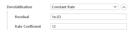
The Constant Rate devolatilization model releases mass at the constant rate:
\(\frac{dm}{dt}=A \cdot m_0\)
where:
- \(\frac{dm}{dt}\) - devolatilization rate
- \(A\) - rate coefficient
- \(m_0\) - initial mass of the volatiles
Inputs:
- Residual - fraction of remaining volatiles, below which combustion can occur
- Rate Coefficient - coefficient determines devolatilization rate
Surface Reaction Models
These models define how char in coal particles is oxidized. Only reactions of the form
\(C+Sb\cdot O_2 \rightarrow CO_2\)
where \(Sb\) is the stoichiometry of the reaction.
Available surface reaction models:
- Kinetic/Diffusion Limited
- Diffusion Limited
- Hurt-Mitchell
Kinetic/Diffusion Limited
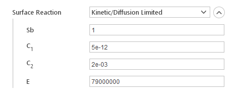
The Kinetic/Diffusion Limited reaction rate is calculated from kinetic rate and limited by diffusion.
Inputs:
- \(Sb\) - stoichiometry of the reaction
- \(C_1\) - mass diffusion limited rate constant
- \(C_2\) - kinetics limited rate pre-exponential constant
- \(E\) - kinetics limited rate activation energy
Diffusion Limited
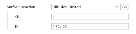
In the Diffusion Limited model, the reaction rate is controlled by diffusion.
Inputs:
- Sb - stoichiometry of the reaction
- D - diffusion coefficient of oxidants
Hurt-Mitchell
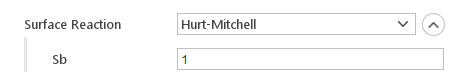
The Hurt-Mitchell model is based on:
                        Hurt R. and Mitchell R.,
  "Unified high-temperature char combustion kinetics for a suite of coals of various rank",
  24th Symposium on Combustion, The Combustion Institute, 1992, p 1243-1250
Inputs:
- Sb - stoichiometry of the reaction
Collision Models
These models define interactions between particles. Available collision models:
- Pair Collision - enables collision between particles and walls. Requires you to specify maximum interaction distance
- Trajectory
- O’Rourke
Pair Collision
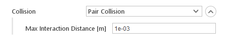
Pair Collision enables collision between particles and walls. Requires specifying maximum interaction distance.
Trajectory Collision
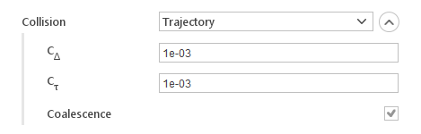
Trajectory collision model check the probability of the collision if at least two parcels are in the same cell. This model take into account the trajectory of each parcel. Collision may happen if parcels are traveling towards each other.
Inputs:
- \(C_{\Delta}\) - spatial collision probability decay
- \(C_{\tau}\) - temporal collision probability decay
- Coalescence - defines whether particles will coalesce after collision or not
O’Rourke Collision
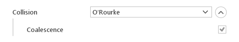
O’Rourke collision model check the number of particles in the same cells and calculate the probability of the collision between them. Algorithm does not take into account trajectory of each parcel. The frequency of the collision increases with smaller cell size.
Inputs:
- Coalescence - defines whether particles will coalesce after collision or not
Pair/Wall Collision Models
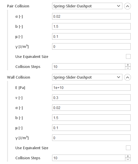
The Pair Collision and Wall Collision models define how particles collide with each other and with the walls. Currently, there is only the Spring-Slider-Dashpot model is available, which assumes that forces during the collision can be modeled using springs, sliders, and dampers.
Inputs:
- \(E [Pa]\) - Young’s modulus of the wall
- \(\nu [-]\) - Poisson’s ratio of the wall
- \(\alpha [-]\) - coefficient related to coefficient of restitution
- \(b [-]\) - spring power (linear: b = 1, Hertzian: b = 3/2)
- \(\mu [-]\) - coefficient of friction in tangential sliding
- \(\gamma [J/m ^3]\) - cohesion energy density
- Use Equivalent Size - use equivalent size particles to reduce computational cost
- Collision Steps - number of steps over which to resolve the collision
Breakup Models
These models define the breakup process of spray droplets. Available breakup models:
- TAB
- ETAB
- Reitz-Diwakar
- Reitz-KHRT
TAB
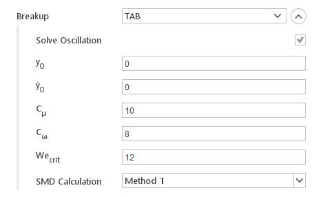
The TAB model is based on:
                        O'Rourke, P.J. and Amsden, A.A.,
  "The TAB Method for Numerical Calculation of Spray Droplet Breakup"
  1987 SAE International Fuels and Lubricants Meeting and Exposition,
  Toronto, Ontario, November 2-5, 1987,
  Los Alamos National Laboratory document LA-UR-87-2105;
  SAE Technical Paper Series, Paper 872089.
ETAB
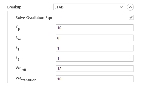
The ETAB model is based on:
                        F.X. Tanner
  "Liquid Jet Atomization and Droplet Breakup Modeling of
  Non-Evaporating Diesel Fuel Sprays"
  SAE 970050,
  SAE Transactions: Journal of Engines, Vol 106, Sec 3 pp 127-140
Reitz-Diwakar
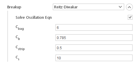
The Reitz-Diwakar model is based on:
                        Reitz, R.D. and Diwakar, R.
  "Effect of drop breakup on fuel sprays"
  SAE Tech. paper series, 860469 (1986)
Reitz, R.D. and Diwakar, R.
"Structure of high-pressure fuel sprays"
SAE Tech. paper series, 870598 (1987)Reitz-KHRT
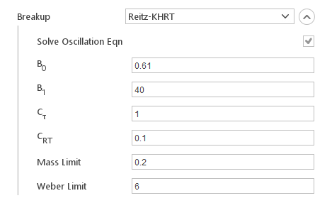
The Reitz-KHRT model is a secondary breakup model which uses the Kelvin-Helmholtz and Raleigh-Taylor instability to predict stripped droplets.
Atomization Models
These models define how continuous phase is converted into droplets. Available atomization models:
- Blob Sheet Atomization
Blob Sheet Atomization Model
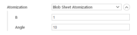
The Blob Sheet Atomization is the primary model for pressure swirl atomizers. It is based on:
                        Z. Han, S. Parrish, P.V. Farrell, R.D. Reitz
  "Modeling Atomization Processes Of Pressure Swirl Hollow-Cone Fuel Sprays"
  Atomization and Sprays, vol. 7, pp. 663-684, 1997
Packing Models
These models describe packing of the particle bed. Available packing models:
- Explicit
- Implicit
Explicit Packing
In this model inter-particle stress is calculated using current particle locations. This force is then applied only to the particles that are moving towards regions of a close pack.
Implicit Packing
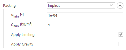
In this model, the time evolution of particulate volume fraction is solved for implicitly on the eulerian mesh. The computed flux is then applied to the lagrangian field. The gravity force can optionally be applied to the particles as part of this model.
Inputs:
- \(\alpha_{min} [-]\) - minimum stable volume fraction
- \(\rho_{min} [-]\) - minimum stable density
- Apply Limiting - whether to apply implicit limiting
- Apply Gravity - apply gravity force
Isotropy Model
These models define how particles return to isotropy after collisions. Available isotropy models:
- Stochastic
Stochastic Isotropy Model
The Stochastic isotropy model is based on:
                        "Inclusion of collisional return-to-isotropy in the MP-PIC method"
  P. O'Rourke and D. Snider
  Chemical Engineering Science
  Volume 80, Issue 0, Pages 39-54, December 2012
Damping Models
These models define damping during particle collision. Available damping models:
- Relaxation - relaxes particle velocities towards the local mean over a time-scale
Particle Stress Model
The Particle Stress model defines inter-particle stress. Available particle stress models:
- Harris-Crighton
- Lun
- Exponential
Harris-Crighton Model
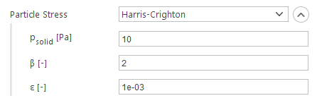
The Harris-Crighton model is based on:
                        "Solitons, solitary waves, and voidage disturbances in gas-fluidized beds"
   S. Harris and D. Crighton,
   Journal of Fluid Mechanics
   Volume 266, Pages 243-276, 1994
Inputs:
- \(p_{solid} [-]\) - solid pressure coefficient
- \(\beta [-]\) - exponent of the volume fraction
- \(\varepsilon [-]\) - the smallest allowable difference from the packed volume fraction
Lun Model
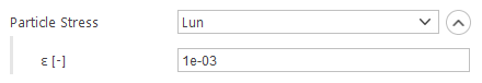
The Lun model is based on:
                        "Kinetic theories for granular flow: inelastic particles in Couette flow and slightly inelastic particles in a general flow field"
  C. Lun, S. Savage, G. Jeffrey, N. Chepurniy
  Journal of Fluid Mechanics
  Volume 140, Pages 223-256, 1984
Inputs:
- \(\varepsilon [-]\) - smallest allowable difference from the packed volume fraction
Exponential Model
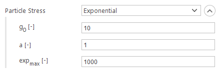
The Exponential model calculates stresses from a simple exponential formula.
Inputs:
- \(g_0 [-]\) - front coefficient
- \(a [-]\) - pre-exponential factor
- \(exp_{max} [-]\) - maximum value of exponent
Time Scale Models
These models define the time scale over which properties of a dispersed phase tend towards the mean value. Available time scale models:
- Equilibrium
- Non-Equlibrium
- Isotropic
Equilibrium Time Scale Model
The Equilibrium model is based on:
                        P. O'Rourke, P. Zhao and D. Snider
  "A model for collisional exchange in gas/liquid/solid fluidized beds"
  Chemical Engineering Science
  Volume 64, Issue 8, Pages 1784-1797, April 2009
Non-Equlibrium
The Non-Equlibrium model is based on:
                        P. O'Rourke and D. Snider
  "An improved collision damping time for MP-PIC calculations of dense particle flows with applications to polydisperse sedimenting beds and colliding particle jets"
  Chemical Engineering Science
  Volume 65, Issue 22, Pages 6014-6028, November 2010
Isotropic
The Isotropic model is based on:
                        P. O'Rourke and D. Snider
  "Inclusion of collisional return-to-isotropy in the MP-PIC method"
  Chemical Engineering Science
  Volume 80, Issue 0, Pages 39-54, December 2012
Correction Limiter Models
These models define how particle velocity correction is limited to improve stability. Available models are:
- Absolute - limits the velocity correction to that of a rebound with a coefficient of restitution, uses absolute velocity
- Relative - limits the velocity correction to that of a rebound with a coefficient of restitution uses relative velocity
Erosion Model
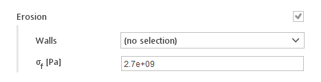
Erosion model creates the particle field on the user-specified patches.
Inputs:
- Walls - patches that are under erosion
- \(\sigma_f [Pa]\) -
Solution
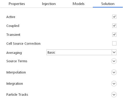
In the Solution tab one can define setting related to the solution of particle motion.
General Settings
At the top of the Solution tab, the basic settings controlling the solution process of the discrete phase are defined.
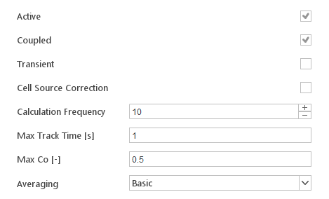
- Active - enable/disable solution process of the discrete phase model
- Coupled - enable/disable coupling between discrete phase and the continuous phase, if coupling is disabled no source terms will be added to continuous phase equations
- Transient - switches between transient and steady-state particle tracking
- Cell Source Correction - correct cell values with latest transfer information during the lagrangian timestep
- Calculation Frequency - (only for steady-state particle tracking) number of continuous phase time steps per discrete phase computation
- Max Track Time [s] - (only for steady-state particle tracking) maximum total track time of a particle
- Max Co [-] - (only for steady-state particle tracking) maximum particle Courant number
- Averaging - lagrangian averaging methods
- Basic - cell-volume based average - values are summed and divided by the cell volume
- Dual - values are summed using the tetrahedral decomposition of the computational cells and the values are weighted by proximity to the cell centre or point
- Moment - values and moments from the cell centroid are summed and the linear function is generated with the same integrated moment as the point data.
Source Term Settings
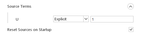
In the Source Terms section one can define how source terms for each continuous phase equation should be computed. They can be computed in an Explicit or Semi-Implicit manner. For each source term, the relaxation factor can be specified. For each source term, the relaxation factor can be specified.
Additionally, the Reset Sources on Startup input can be used to indicate whether coupling source terms should be reset on start-up.
Interpolation Settings
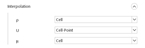
In the Interpolation section one can define how each field value from the continuous phase is interpolated to the current location of the particle. Currently, available interpolation schemes:
- Cell - uses cell value for any point inside the cell
- Cell-Point - uses cell values and node values and performs linear interpolation between them
- Cell-Point-Face - uses cell values, face values and node values and performs linear interpolation between them
Integration Settings
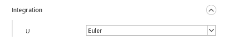
In the Integration section one can define how each of the particle values is integrated. Available integration methods:
- Analytical - integrate analytically
- Euler - integrate using the implicit Euler method
Particle Tracks Settings
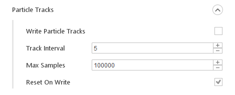
In the Particle Tracks section, one can configure how particle tracks are stored. Storing particle tracks is only available when using steady-state particle tracking. Options to define particle tracks:
- Write Particle Tracks - enable or disable writing of the particle tracks
- Track Interval - number of face-hit intervals between storing data
- Max Samples - maximum number of particles to store per track
- Reset On Write - whether data should be cleared on writing