Dynamic Mesh
Introduction
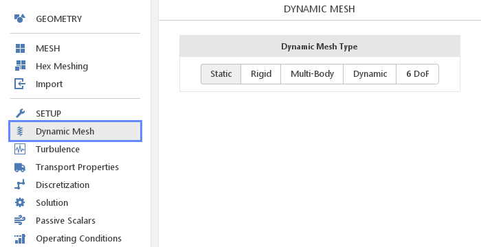
In the Dynamic Mesh panel, models for moving and deforming the mesh are defined. Besides, the Static model representing the lack of any motion, currently available dynamic mesh models are:
- Rigid
- Multi-Body
- Dynamic
- 6DoF
Rigid Body Motion
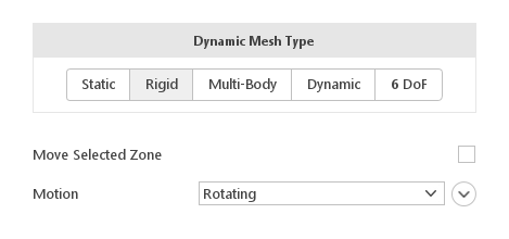
The Rigid dynamic mesh type allows moving the mesh according to a prescribed motion function. Optionally, the motion can only be applied to a selected cell zone. Note that this model does not allow for any deformation, just rigid body motion.
Moving Selected Zone
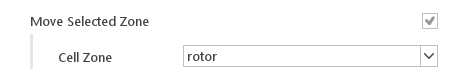
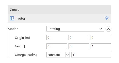
When your mesh contains cell zones, the Move Selected Zone checkbox will be active, allowing you to apply motion only to selected Cell Zone . This option is typically used for modeling turbomachinery, where you typically have some static and some rotating parts.
Motion Functions
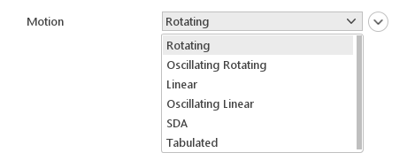
The Motion input defines what type of motion will be applied to the mesh or the selected cell zone.
Rotating Motion
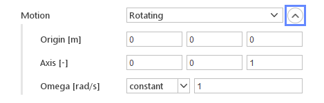
The Rotating motion function rotates the mesh about a prescribed axis at a defined speed.
Inputs:
- Origin [m] - the point around which the rotation should occur
- Axis - rotation axis vector
- Omega [rad/s] - rotational speed (may vary in time)
Oscillating Rotating Motion
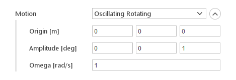
The Oscillating Rotating motion defines a simple angular oscillation where rotation angle is described as:
\(\varphi (t)=A \cdot sin(\omega t)\)
where:
- \(\varphi (t)\) - intentenous value of the rotation angle
- \(A\) - oscillation amplitude
- \(\omega\) - oscillation speed
- \(t\) - time
Inputs:
- Origin [m] - the point around which the rotation should occur
- Amplitude [deg] - amplitude of the rotation
- Omega [rad/s] - rotational speed
Note that the Amplitude input also defines the rotation axis.
Linear Motion
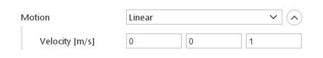
The Linear motion simply moves the mesh at a constant velocity.
Inputs:
- Velocity [m/s] - velocity of the mesh
Oscillating Linear Motion
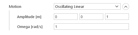
The Oscillating Linear motion defines a simple linear oscillation where mesh position is described as:
\(x(t)=A \cdot sin( \omega t) x(t) = A \cdot sin( \omega t)\)
where:
- \(x(t)\) - instantenous position
- \(A\) - oscillation amplitude
- \(\omega\) - oscillation speed
- \(t\) - time
Inputs:
- Amplitude [m] - amplitude of the oscillation
- Omega [rad/s] - rotational speed
Note that the Amplitude input also defines the direction of the motion.
Ship Design Analysis (SDA) Motion
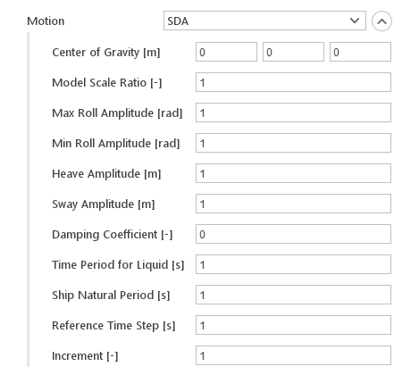
The SDA motion is a three degree of freedom motion function, comprising sinusoidal roll (rotation about X axis), heave (translation in the Z direction) and sway (translation in the Y direction) motions with changing amplitude and phase.
Inputs:
- Center of Gravity [m]
- Model Scale Ratio [-]
- Max Roll Amplitude [rad]
- Min Roll Amplitude [rad]
- Heave Amplitude [m]
- Sway Amplitude [m]
- Damping Coefficient []
- Time Period for Liquid [s]
- Ship Natural Period [s]
- Reference Time Step [s]
- Increment [-]
Tabulated Motion
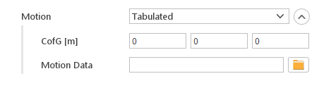
Tabulated motion allows importing external motion data.
Inputs:
- Center of Gravity [m]
- Motion Data - external file should contain the overall number of data sets, time and displacement vector for each set
Multi-Body
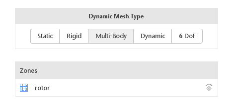
The Multi-Body dynamic mesh type is similar to Rigid , but it allows for defining different motion functions in each cell zone. Also, it does not allow for moving the entire mesh directly. Options for this panel consists of a cell zone list where individual motion functions can be defined.
Applying Motion Functions
To apply motion function to a cell zone you need to click on the cell zone name in the Zones list. Options for selected zone will be displayed below the list. In the displayed options you just need to select Motion function similarly to what is done for Rigid model.
Dynamic Motion
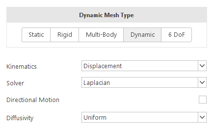
The Dynamic mesh type allows you to move or deform boundaries. Boundary motion can be described upfront as well as they can be computed dynamically based on the current solution state. The definition of boundary motion is done, like in the case of other models, in the Boundary Conditions panel.
Motion Kinematics
The Kinematics input specifies how the boundary motion is defined. There are two options:
- Displacement - you define how the displacement of the boundary changes in time
- Velocity - you define how the velocity of the boundary changes in time
Mesh Deformation Solver
The Solver input defines which technique should be used to interpolate boundary motion into internal mesh deformation. There are currently two solvers available:
- Laplacian
- SBR Stress
Laplacian Displacement Solver
The Laplacian solver translates boundary deformation into internal mesh deformation by solving the Laplace equation:
\(\nabla\cdot(D\cdot\nabla\Delta)=0\)
where:
- \(\Delta\) - mesh deformation or velocity
- \(D\) - deformation diffusivity
Solid-body Rotation Stress Solver
The SBR Stress solver calculates mesh displacement by solving the cell-centre solid-body rotation stress equations of the form:
\(\nabla\cdot D(\nabla \Delta + (\nabla \Delta)T -tr(\nabla \Delta))=0\)
where:
- \(\Delta\) - mesh deformation
- \(D\) - deformation diffusivity
Note that this solver can only be used when displacement kinematics is selected.
Directional Motion

You can enable Directional Motion input if you want to constraint motion to a specific direction. Then you will have to select one of the directions of global coordinate system.
Motion Diffusivity
Diffusivity controls how much boundary motion influences the internal mesh. Where the diffusivity is high, the deformations at the boundary strongly influence the internal mesh, when the diffusivity is low only mesh near the boundary is deforming. This input is used by both Laplacian and SBR Stress solver. Currently, available diffusivity models are:
- Uniform
- Directional
- Inverse Distance
- Inverse Volume
Uniform Diffusivity
The Uniform diffusivity model assumes that it is constant inside the domain. Equations solved by the Laplacian and SBR Stress are such that when diffusivity is uniform, its value is not important, therefore you do not have to specify a value.
Directional Diffusivity

The Directional diffusivity model allows for diffusivity to be different in every direction of the global coordinate system.
Inputs:
- Diffusivity Directions - value of diffusivity in each direction of the global coordinate system
Inverse Distance Diffusivity
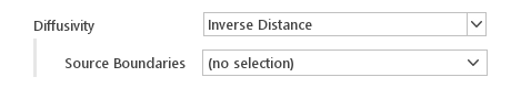
In the Inverse Distance diffusivity model, the diffusivity is proportional to the inverse of the distance from the selected boundaries.
Inputs:
- Source Boundaries - boundaries, distance from which is taken to calculate the diffusivity
Inverse Volume Diffusivity
The Inverse Volume model calculates diffusivity by taking the inverse of the volume of the cell for which the diffusivity is calculated.
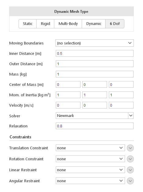
Six Degrees of Freedom
The 6 DoF solver will predict the trajectory of a moving body using the aero or hydrodynamic forces and inertial properties assigned to a given boundary. During the analysis, the mesh will adjust to the new position of the body by moving nodes in the deformation region defined by the distance from the body. Additionally, you have the possibility to apply various constraints to the boundary motion.
Moving Boundaries
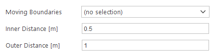
The Moving Boundaries input specifies which boundaries should be moving according to the solution of motion equations. Additionally, you will have to specify Inner Distance and Outer Distance from the boundaries. Mesh nodes within the Inner Distance will move exactly like the boundaries. Mesh nodes outside the Outer Distance will not move at all.
Boundaries Properties
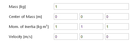
To be able to solve motion equations the solver requires mass properties of moving boundary.
Inputs:
- Mass [kg] - mass of the body
- Center of Mass [m] - coordinates of the center of mass
- Mom of Inertia [kg m2] - moment of inertia
- Velocity [m/s] - body velocity
Solver
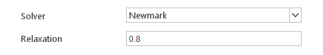
Two solvers are available:
- Newmark
- CrankNicolson
Additionaly we can set the Relaxation parameter to control convergence process.
Constraints
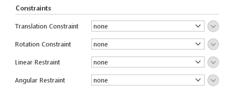
It is possible to constrain or restraint boundary motion.
Translation Constraint
We distinguish 3 types of Translation Constraint:
- Linear - body can move along one direction - rest DoFs are fixed

- Plane - body can move on the selected plane which is defined by the normal vector

- Point - translation relative to the selected point is fixed

Rotation Constraint
Rotation Constraints allow to fixed the body rotation. There is two type of constraint:
- Axis - rotation around the selected axis is fixed
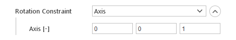
- Fix Orietation - all rotation degree of freedom are fixed
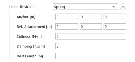
Linear Restraint
Restraint options
- Damper
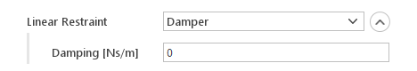
- Spring
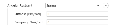
Angular Restraint
- Damper

- Spring