Radiation
Introduction
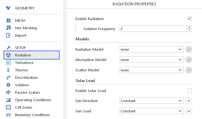
In the Radiation panel, you can define settings related to radiation modelling.
Enabling Radiation

Radiation models can be very computationally expensive, to reduce the simulation time you can take advantage of a few options.
The Enable Radiation input allows you to enable or disable radiation computation when it might not be necessary. In a typical situation, when doing a steady-state simulation, you would disable radiation during initial iterations when the flow field is very different from the final solution and computing costly radiation might not be beneficial. After the flow field starts to converge you can enable radiation, to get correct results with a minimal cost.
The Solution Frequency input provides similar benefits. It allows you to solve costly radiation equations only every N-th iteration. This can be beneficial since usually the flow field changes slowly from iteration to iteration and computing radiation in every step can be wasteful. This means that you are mostly using radiation sources computed from an older iteration. However, when the simulation converges, the flow fields stops to change and the radiation becomes practically up-to-date.
Radiation Modeling
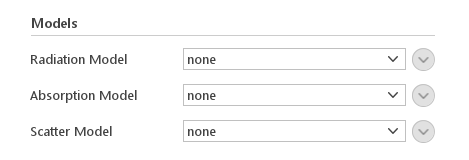
There are three basic models you need to define to fully describe radiation. The three models are:
- Radiation
- Absorption
- Scatter
Each of the models has a default value none , which indicates that no modelling should be used for this aspect of radiation.
Radiation Models

Radiation Model is what actually computes the influence of radiation on energy balance in the domain.
Available models are:
- P1
- Discrete Ordinates
- Surface to Surface
P1 Radiation Model
The P1 model is the simplest case of the more general PN model, which is based on the expansion of the radiation intensity \(I\) into an orthogonal series of spherical harmonics. It calculates radiative heat flux from the following expressions:
\(q_r=-\Gamma \nabla G\)
\(\Gamma=1/{3(a+\sigma_{eff})}\)
where:
- \(q_r\) - radiative heat flux
- \(G\) - incident radiation
- \(a\) - absorbtion coefficient
- \(\sigma_{eff}\) - effective scattering coefficient
Incident radiation \(G\) is calculated from the following equation:
\(\nabla \cdot (\Gamma \nabla G) -a G=-4e \sigma T^4 \)
where:
- \(\sigma\) - Stefan-Boltzmann constant
- \(e\) - emission coefficient
- \(T\) - temperature
The model is very computationally inexpensive. However, it should only be applied for models with large optical thickness ( \(\tau =aL>3\), where \(L\) is the distance between objects). Additionally, it assumes that all surfaces are diffuse, and it tends to over predict radiative fluxes from localised heat sources and sinks
Discrete Ordinates Radiation Model
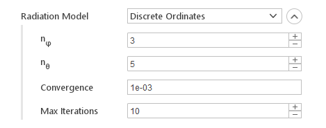
The Discrete Ordinates radiation model solves the radiative transfer equation for a finite number of directions in a participating medium without scatter. You define the number of directions by specifying the angular discretization. The model calculates radiation intensity by solving, for each of the directions, equations of the form:
\(\nabla \cdot (I(\vec s )\vec s) +aI(\vec s)=1 \pi (a \sigma T^4 -E/4)\)
where:
- \(\vec s\) - direction vector
- \(I(\vec s)\) - radiation intensity in the directions \(\vec s\)
- \(E\) - net emission contribution
- \(\sigma\) - Stefan-Boltzmann constant
- \(a\) - absorption coefficient
- \(T\) - temperature
Inputs:
- \(n_\varphi\) - number of divisions in the azimuthal direction
- \(n_\theta\) - number of divisions in the polar direction
- Convergence - convergence criteria for radiation equations
- Max Iterations - maximum number of iterations when solving radiation equations
Note: Increasing the number of divisions in each angular direction will very rapidly increase the computational cost. Use it with care.
Surface to Surface Radiation Model
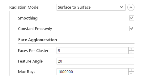
The Surface to Surface radiation model uses view factors to compute radiative heat fluxes between boundaries. To reduce computational cost, view factors are not computed for each individual mesh face, but faces are grouped in clusters of a specified size.
Inputs:
- Smoothing - perform view factor matrix smoothing
- Constant Emmisivity - perform optimisations for uniform emissivity
- Faces Per Cluster - number of faces in a face cluster
- Feature Angle - geometry feature angle
- Max Rays - maximum number of rays to use when calculating view factors
Absorption Models
The Absorption model provide absorption and emission coefficients that are used by radiation models. Currently, available models:
- Constant
Constant Absorption/Emission Model

The Constant model assumes that absorption and emission coefficient are fixed.
Inputs:
- \(a [1/m]\) - (absorptivity) absorption coefficient
- \(e [1/m]\) - (emissivity) emission coefficient
- \(E [{kg}/m s^3]\) - emission contribution
Scatter Model
The Scatter model provides radiation scattering coefficients. Currently available models:
- Constant
Constant Scatter Model

The Constant model assumes constant scattering coefficient with optional anisotropy.
Inputs:
- \(\sigma [1/m]\) - scattering coefficient
- \(C [-]\) - linear-anisotropic phase function coefficient
Solar Load Modeling
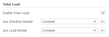
You have an option to add Solar Load to your simulation. This model introduces additional radiation source that can be used to simulate solar radiation. When you Enable Solar Load you need to specify models for:
- Sun Direction
- Sun Load
Note: Solar Load model is only available when you are using the Plus version of OpenFOAM.
Sun Direction

The Sun Direction model defines from which direction the solar radiation is coming from. Available models are:
- Constant
- Sun Tracking
Constant Sun Direction

The Constant model assumes that the sun is “fixed” in the sky. This approach can be useful when the time scales of the simulations are small compared to the time scales of the sun motion.
Inputs:
- Direction - direction from which the solar radiation is incoming
Sun Tracking
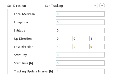
The Sun Tracking model calculates the current sun position from local time, coordinates and mesh orientation. This model can only be used in transient simulations.
Inputs:
- Local Meridian - Local Zone Meridian in hours
- Longitude - longitude in degrees
- Latitude - latitude in degrees
- Up Direction - up direction of the mesh
- East Direction - east direction of the mesh
- Start Day - start day of the simulation
- Start Time - start time of the simulation in hours
- Tracking Update Interval - interval for updating sun direction
Sun Load Modelling
The Sun Load models defines how much radiative energy is applied from the sun. Currently, available models:
- Constant
Constant Load Model

The Constant sun load model assumes fixed values for direct and diffuse energy fluxes from the sun.
Inputs:
- Direct - direct energy flux
- Diffuse - diffuse energy flux