Thermo
Introduction
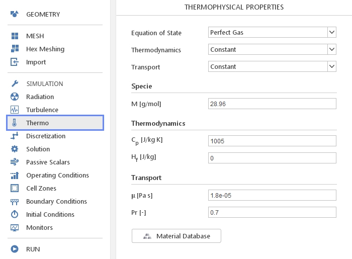
In the Thermo panel, you can define thermophysical properties of your material. In contrast to the Transport Properties panel, here you define material properties for compressible flow solvers.
Material Models
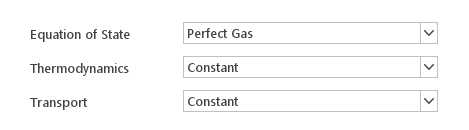
To fully describe material properties for compressible simulations you need to define three material models:
- Equation of State
- Thermodynamics
- Transport
Available material models will depend on selected solver. Additionally, not all combinations of these models are available, which means that when you change the Equation of State , the list of Thermodynamics and Transport models will change.
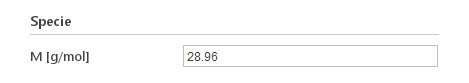
Besides the models, you need to specify molar mass of your material under Specie input group.
Equations of State
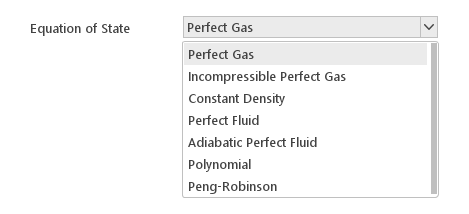
Equation of State model defines the relationship between parameters of state: density, pressure, and temperature. Available equations of state depend on a currently selected solver and, in the case of the multi-region solvers, on whether mesh region is solid or fluid.
Available Equations of State:
- Perfecte Gas
- Incompressible Perfect Gas
- Constant Density
- Perfect Fluid
- Adiabatic Perfect Fluid
- Peng-Robinson
- Polynomial
Perfect Gas
The Perfect Gas equation of state describes the behaviour of a hypothetical perfect gas , which is a good approximation for real gases under moderate pressures. It can be expressed as:
\(\rho=\frac{p}{R \cdot T}\)
where:
- \(\rho\) - density
- \(p\) - pressure
- \(R\) - specific gas constant
- \(T\) - temperature
The only constant in this equation is \(R\) which can be calculated from universal gas constant and molar mass, therefore the Perfect Gas equation of state does not require additional inputs.
Incompressible Perfect Gas
The Incompressible Perfect Gas equation of state uses a constant reference pressure in the perfect gas equation of state rather than the local pressure so that the density only varies with temperature and composition. It can be expressed as:
\(\rho=\frac {p_{ref}}{R \cdot T}\)
where:
- \(\rho\) - density
- \(p_{ref}\) - reference pressure
- \(R\) - specific gas constant
- \(T\) - temperature
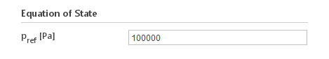
Inputs:
- \(p_{ref} [Pa]\) - reference pressure
Constant Density
The Constant Density equation of state assumes that density is constant:
\(\rho = const\)
where:
- \(\rho\) - density
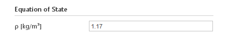
Inputs:
- \(\rho [{kg}/m^3]\) - density
Perfect Fluid
The Perfect Fluid equation of state calculates density using the following expression:
\(\rho=\rho_0 +\frac{p}{R \cdot T}\)
where:
- \(\rho\) - density
- \(\rho_0\) - reference density
- \(p\) - pressure
- \(R\) - specific gas constant
- \(T\) - temperature
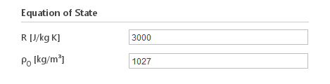
Inputs:
- \(R [J/{kg} K]\) - "specific gas constant"
- \(\rho_0 [{kg}/m^3]\) - reference density
Note: The "specific gas constant" needs to be explicitly specified since it cannot be computed from molar mass using perfect gas laws.
Adiabatic Perfect Fluid
The Adiabatic Perfect Fluid equation of state calculates density using the following expression:
\(\rho=\rho_0 \cdot (\frac{p+B}{p_0 +B})^{\frac{1}{\gamma}}\)
where:
- \(\rho\) - density
- \(\rho_0\) - reference density
- \(p\) - pressure
- \(p_0\) - reference pressure
- \(B\) - universal gas constant
- \(\gamma\) - adiabatic expansion constant
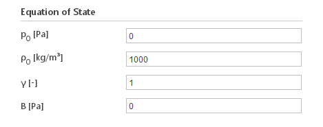
Inputs:
- \(p_0 [Pa]\) - reference pressure
- \(\rho_0 [{kg}/m^3]\) - reference density
- \(\gamma [-]\) - adiabatic expansion constant
- \(B [Pa]\) - universal gas constant
Peng-Robinson
The Peng-Robinson equation of state is a better approximation of the behaviour of real gases than the Perfect Gas . It is expressed using the following relations:
\(p=\frac{BT}{V_m-b}-\frac{a \alpha}{ V_m^2+2bV_m-b^2}\)
\(a \approx 0.45724 \cdot \frac{B^2 T_c ^2}{p_c}\)
\(b \approx 0.07780 \cdot \frac{B T_c }{p_c}\)
\(\alpha = (1+\kappa(1- T_r^{1/2}))^2\)
\(\kappa \approx 0.37464 + 1.54226 \omega - 0.26992 \omega^2\)
\(T_r=\frac{T}{T_c}\)
where:
- \(p\) - pressure
- \(T\) - temperature
- \(V_m\) - molar volume
- \(T_c\) - temperature at critical
- \(p_c\) - pressure at critical
- \(V_c\) - molar volume at critical
- \(\omega\) - acentric factor
- \(B\) - universal gas constant
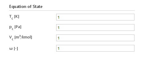
Inputs:
- \(T_c [K]\) - temperature at critical point
- \(p_c [Pa]\) - pressure at critical point
- \(V_c [m^3/{kmol}]\) - molar volume at critical point
- \(\omega [-]\) - acentric factor
Polynomial
The Polynomial equation of state calculates density using a polynomial function:
\(\rho = \Sigma_{i = 0}^{n} a_1 \cdot T^i\)
where:
- \(\rho\) - density
- \(T\) - temperature
- \(a_i\) - polynomial coefficients
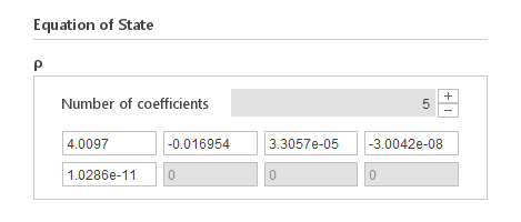
Inputs:
- \(a_i [ \frac{kg}{m^{3} \cdot T^{-i}}]\) - polynomial coefficients
Thermodynamics Models
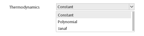
The Thermodynamics models define the relationship between basic parameters of state (pressure and temperature) and derived secondary parameters of state such as enthalpy, entropy and internal energy.
Available Thermodynamics Model:
- Constant
- Polynomial
- Janaf
Constant
The Constant thermodynamics model defines specific heat to be constant:
\(C_p=const\)
where:
- \(C_p\) - specific heat under constant pressure
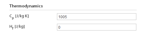
Inputs:
- \(C_p [J/{kg} K]\) - specific heat under constant pressure
- \(H_f [J/{kg}]\) - enthalpy of formation
Polynomial
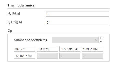
The Polynomial model calculates specific heat using a polynomial function:
\(C_p=\Sigma _{i = 0}^n a_1 \cdot T^i \)
where:
- \(C_p\) - specific heat under constant pressure
- \(T\) - temperature
- \(a_i\) - polynomial coefficients
Inputs:
- \(H_f [J/{kg}]\) - enthalpy of formation
- \(S_f [J/{kg} K]\) - standard entropy
- \(a_i [ 1/{kg} T^{-1-i}]\) - polynomial coefficients
Janaf
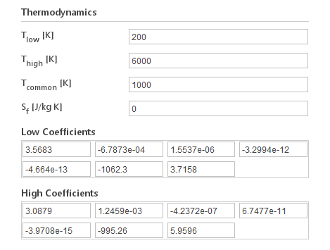
The Janaf model calculates specific heat as a function of temperature using coefficients from JANAF tables of thermodynamics. Two sets of coefficients need to be specified, the first set for temperatures below a common temperature, the second for temperatures above common temperature. The formula for calculating specific heat is:
\(C_p =R \cdot \Sigma_{i=0}^4 a_i \cdot T^i\)
where:
- \(C_p\) - specific heat under constant pressure
- \(R\) - gas constant
- \(a_i\) - JANAF coefficients
Inputs:
- \(T_{low} [K]\) - low temperature limit for model aplicability
- \(T_{high} [K]\) - high temperature limit for model aplicability
- \(T_{common} [K]\) - temperature delimiter for when to use low or high coefficient
- \(a_i [K^-i]\) (lowCpCoeffs/highCpCoeffs) \([K^{-1}]\) - JANAF coefficients
Transport Models
The Transport models define thermal conductivity and viscosity which are later used in transport equations for momentum and energy.
Available Transport Models:
- Constant
- Sutherland
- Polynomial
Constant
The Constant transport model assumes that transport properties are constant. In this model thermal conductivity is calculated using the formula:
\(\kappa = \frac{C_p \cdot \mu}{P_r}\)
where:
- \(\kappa\) - thermal conductivity
- \(C_p\) - specific heat under constant pressure
- \(\mu\) - dynamic viscosity
- \(P_r\) - Prandtl number
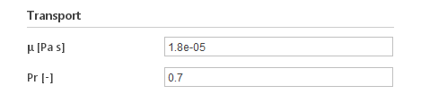
Inputs:
- \(\mu [Pa \cdot s]\) - dynamic viscosity
- \(P_r [-]\) - Prandtl number
Sutherland
The Sutherland model calculates dynamic viscosity from the Sutherland formula:
\(\mu=\frac{A_s T^{0.5}}{1+\frac{T_s}{T}}\)
where:
- \(\mu\) - dynamic viscosity
- \(T\) - temperature
- \(A_s\) - Sutherland coefficients
- \(T_s\) - Sutherland temperature
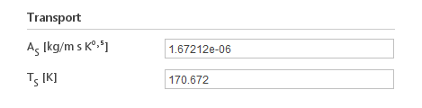
Inputs:
- \(A_s [{kg}/m s K ^0.5 ]\) - Sutherland coefficients
- \(T_s [K]\) - Sutherland temperature
Polynomial
The Polynomial transport model calculates dynamic viscosity and thermal conductivity from polynomial expressions:
\(\mu=\Sigma_{i=0}^n a_{\mu i} \cdot T^i\)
\(\kappa=\Sigma_{i=0}^n a_{\kappa i} \cdot T^i\)
where:
- \(\mu\) - dynamic viscosity
- \(\kappa\) - thermal conductivity
- \(T\) - temperature
- \(a_{x i}\) - polynomial coefficients
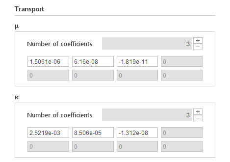
Inputs:
- \(a_{\mu i} [Pa s K ^-i ]\) - dynamic viscosity polynomial coefficients
- \(a_{x i} [W/m K ^{1+i} ]\) - thermal conductivity polynomial coefficients
Cavitation Properties
When you select a cavitation solver a set of properties specific to this solver will be displayed.
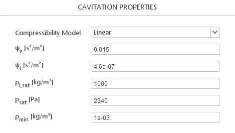
Compressibility Models
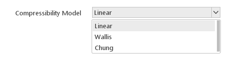
Cavitation properties require you to define a Compressibility Model that describes compressibility of the mixture.
Available Compressibility Models:
- Linear
- Wallis
- Chung
Linear Model
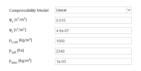
The Linear model defines mixture compressibility as linear combination of vapour and liquid compressibilities:
\(\psi=\gamma \cdot \psi_v +(1-\gamma)\cdot \psi_l\)
where:
- \(\psi\) - mixture compressibility
- \(\psi_v\) - vapour compressibility
- \(\psi_l\) - liquid compressibility
- \(\gamma\) - vapour phase fraction
Inputs:
- \(\Psi_v [s^2/m^2]\) - vapour compressibility
- \(\Psi_l [s^2/m^2]\) - liquid compressibility
Wallis Model
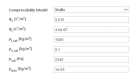
The Wallis model computes mixture compressibility using the following equations:
\(\psi =(\gamma \rho_{v,sat} + (1-\gamma) \rho_{l,sat})(\gamma \frac{\psi_v}{ \rho_{v,sat}}+(1-\gamma)\frac{\psi_l}{ \rho_{l,sat}})\)
where:
- \(\psi\) - mixture compressibility
- \(\psi_v\) - vapour compressibility
- \(\psi_l\) - liquid compressibility
- \(\rho_{v,sat}\) - vapour saturation density
- \(\rho_{l,sat}\) - liquid saturation density
- \(\gamma\) - vapour phase fraction
Inputs:
- \(\Psi_v [s^2/m^2]\) - vapour compressibility
- \(\Psi_l [s^2/m^2]\) - liquid compressibility
- \(\rho_{v,sat} [{kg}/m^3]\) - vapour saturation density
- \(\rho_{l,sat} [{kg}/m^3]\) - liquid saturation density
Chung Model

The Chung model computes mixture compressibility using the following equations:
\(s_{fa} = \frac{\frac{\rho_{v,sat}}{\psi_v}}{(1-\gamma)\frac{\rho_{v,sat}}{\psi_v}+ \gamma \frac{\rho_{l,sat}}{ \psi_l}}\)
\(\psi=((\frac{1-\gamma}{ \sqrt{\psi_v}} + \frac{\gamma s_{fa}}{\sqrt{\psi_l}}) \frac{\sqrt{\psi_v \psi_l}}{s_{fa}})^2\)
where:
- \(\psi\) - mixture compressibility
- \(\psi_v\) - vapour compressibility
- \(\psi_l\) - liquid compressibility
- \(\rho_{v,sat}\) - vapour saturation density
- \(\rho_{l,sat}\) - liquid saturation density
- \(\gamma\) - vapour phase fraction
Inputs:
- \(\Psi_v [s^2/m^2]\) - vapour compressibility
- \(\Psi_l [s^2/m^2]\) - liquid compressibility
- \(\rho_{v,sat} [{kg}/m^3]\) - vapour saturation density
- \(\rho_{l,sat} [{kg}/m^3]\) - liquid saturation density
Region Properties
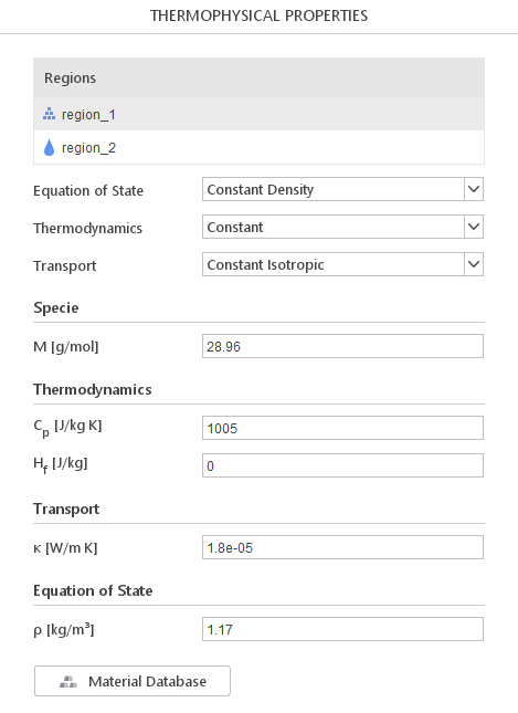
When you select a multi-region, a list of regions will be displayed. By clicking on region name, you will be able to define properties for this region. The definition of material models for each region is the same as in single-region solvers.
Phase Properties
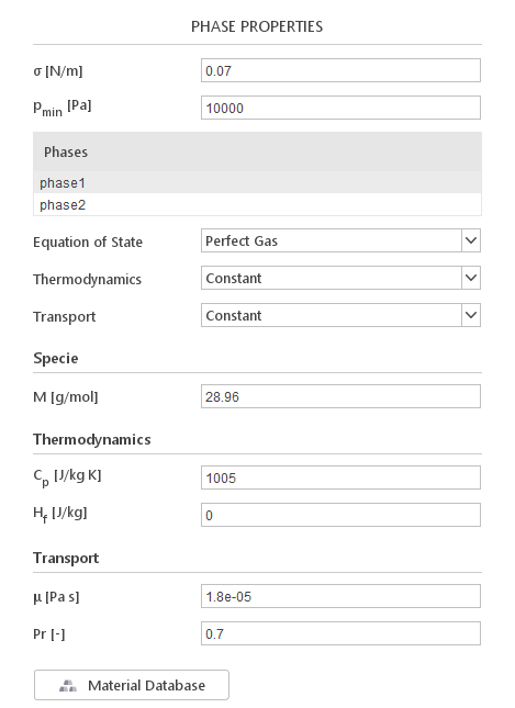
When you select a multiphase solver, a list of current phases will be displayed. When you select a phase in the list, transport properties for this phase will be displayed below.
Additionally, to individual phase properties, you need to define additional values:
- \(\sigma [N/m]\) - surface tension between the phases
- \(\rho_{min} [Pa]\) - lower limit for pressure
Material Database
You can load material properties from the database in a way described for Transport Properties panel.