Transport Properties
Introduction
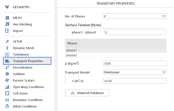
In the Transport Properties panel, you can define transport properties for materials used in incompressible simulations. Here you also define properties of each phase in a multiphase simulation, as well as interactions between those phases.
Standard Material Properties
Depending on selected solver, set of properties you need to define will vary. In general, you will have to specify a subset of available properties:
- \(\beta [\frac{1}{K}]\) - thermal expansion
- \(D_T[\frac{m^2}{s}]\) - thermal diffusion coefficient
- \(\rho[\frac{kg}{m^3}]\) - density
- \(\nu[\frac{m^2}{s}]\) - kinematic viscosity
- \(\mu[Pa \cdot s]\) - dynamic viscosity
- \(\kappa[\frac{W}{m \cdot K}]\) - thermal conductivity
- \(C_p[\frac{J}{kg \cdot K}]\) - specific heat under constant pressure
- \(C_v[\frac{J}{kg \cdot K}]\) - specific heat under constant volume
- \(R[\frac{J}{kg \cdot K}]\) - specific gas constant
- \(H_f[\frac{J}{kg}]\) - enthalpy of formation
- \(S_f[\frac{J}{kg \cdot K}]\) - standard state entropy
- \(M[\frac{g}{mol}]\) - molar mass
- \(Pr[-]\) - Prandtl number
- \(Pr_t[-]\) - turbulent Prandtl number
- \(T_{ref}[K]\) - reference temperature
- \(p_{ref}[Pa]\) - reference pressure
- \(\rho_{ref}[\frac{kg}{m^3}]\) - reference density
- \(C_{p,ref}[\frac{J}{kg \cdot K}]\) - reference specific heat
- \(A_S[\frac{kg}{m \cdot s \cdot K^{0.5}}]\) - Sutherland coefficient
- \(T_S[K]\) - Sutherland temperature
- \(T_{low}[K]\) - low Janaf temperature limit
- \(T_{high}[K]\) - high Janaf temperature limit
- \(T_{common}[K]\) - common Janaf temperature
- \(p_{v,sat}[Pa]\) - saturation pressure
- \(\rho_{v,sat}[\frac{kg}{m^3}]\) - vapour saturation density
- \(\rho_{l,sat}[\frac{kg}{m^3}]\) - liquid saturation density
- \(\Psi_v[\frac{s^2}{m^2}]\) - kinematic vapour compressibility
- \(\Psi_l[\frac{s^2}{m^2}]\) - kinematic liquid compressibility
Transport Model
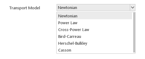
Most incompressible flow solvers require you to specify Transport Model . Transport model specifies how viscosity depends on shear rate \(\dot \gamma\)
Available Transport Models:
- Newtonian
- Power Law
- Cross-Power Law
- Bird-Carreau
- Herschel-Bulkley
- Casson
Newtonian Model

The Newtonian model describes viscosity of a Newtonian fluid , which means that viscosity does not depend on shear rate.
Inputs:
- \(\nu [\frac{m^2}{s}]\) - kinematic viscosity
Power Law Model
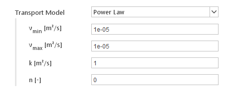
The Power Law model describes viscosity of a power-law fluid defined as:
\(\nu=k \cdot \dot \gamma^{n-1}\)
where:
- \(k\) - flow consistency index
- \(n\) - flow behavior index
Implementation of this model is additionally constraint, so that the computed viscosity is bound between specified minimum and maximum value.
Inputs:
- \(\nu_{min} [m^2/s]\) - minimum kinematic viscosity
- \(\nu_{max} [m^2/s]\) - maximum kinematic viscosity
- \(k [m^2/s^{1-n}]\) - flow consistency index
- \(n[-]\) - flow behavior index
Cross-Power Law Model
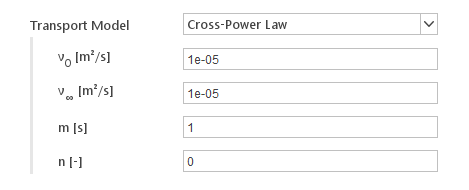
The Power Law model describes viscosity of a Cross fluid defined as:
\(\nu=\nu_\infty + \frac{\nu_0 - \nu_\infty}{1+(m \cdot \dot \gamma)^n}\)
where:
- \(\nu_0\) - viscosity at zero shear rate
- \(\nu_\infty\) - viscosity at infinite shear rate
- \(m\) - relaxation time
- \(n\) - power index
Inputs:
- \(\nu_0 [m^2/s]\) - kinematic viscosity at zero shear rate
- \(\nu_\infty [m^2/s]\) - vkinematic iscosity at infinite shear rate
- \(m [s]\) - relaxation time
- \(n[-]\) - power index
Bird-Carreau Model
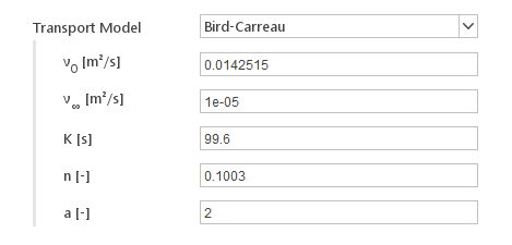
The Bird-Carreau model describes viscosity of a Carreau fluid using Bird-Carreau-Yasuda formulation:
\(\nu=\nu_\infty + \frac{\nu_0 - \nu_\infty}{(1+(k \cdot \dot \gamma)^a )^{\frac{n-1}{a}}}\)
where:
- \(\nu_0\) - viscosity at zero shear rate
- \(\nu_\infty\) - viscosity at infinite shear rate
- \(m\) - relaxation time
- \(n\) - power index
- \(a[-]\) - Yasuda coefficient, determines how quickly viscosity transitions from \(\nu_0\) to \(\nu_\infty\)
Inputs:
- \(\nu_0 [m^2/s]\) - kinematic viscosity at zero shear rate
- \(\nu_\infty [m^2/s]\) - vkinematic iscosity at infinite shear rate
- \(m [s]\) - relaxation time
- \(n[-]\) - power index
- \(a[-]\) - Yasuda coefficient
Herschel-Bulkley Model
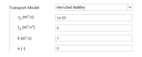
The Herschel-Bulkley model represents viscosity of a Herschel-Bulkley fluid described by:
\(\nu = \{ \begin{matrix} \nu_0 & \dot \gamma \leq \dot \gamma_0 \\ k\cdot |\dot\gamma| ^{n-1}+\tau_0\cdot |\dot\gamma| ^{n} & \dot \gamma > \dot \gamma_0 \end{matrix}\)
where:
- \(\nu_0\) - viscosity at zero shear rate
- \(\tau_0\) - yield stress
- \(k\) - flow consistency index
- \(n\) - flow behavior index
- \(\dot\gamma_0\) - critical shear rate
Inputs:
- \(\nu_0[m^2/s]\) - kinematic viscosity at zero shear rate
- \(\tau_0[m^2/s^2]\) - kinematic yield stress
- \(k[m^2/s^{1-n}]\) - consistency index
- \(n[-]\) - flow index
Casson Model
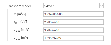
The Casson model specifies minimum and maximum viscosities. Beyond a threshold in strain-rate \(\tau_0\), the viscosity is described by a relationship:
\(\nu = (\sqrt{\frac{\tau_0}{\dot \gamma}} + \sqrt{m})^2\)
Inputs:
- \( m[m^2/s]\) - consistency index
- \(\tau_0[m^2/s^2]\) - kinematic yield stress
- \(\nu_{min}[m^2/s]\) - the minimum value of viscosity in shear thickening fluid
- \(\nu_{max}[m^2/s]\) - the maximum value of viscosity in shear thickening fluid
Phase Properties
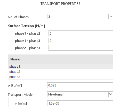
When you select a multiphase solver, in the Transport panel, a list of current phases will be displayed. When you select a phase in the list, transport properties for this phase will be displayed below.
Phase Interactions
For multiphase solvers, besides properties for each individual phase, you will have to define interactions between the phases. Each solver models phase interactions in a different manner and therefore requires a different set of inputs.
Drift Flux Foam Solver

When you select Drift Flux solver you will have to define a model for relative velocity between the continuous and dispersed phase.
Relative Velocity Models:
- Simple
- General
Simple Model
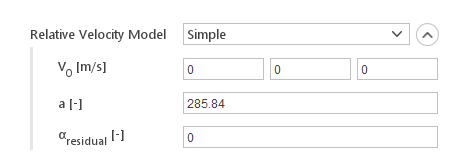
The Simple relative velocity model calculates dispersed diffusion velocity using the formula:
\(U_d=\frac{\rho_c}{\rho}\cdot V_0 \cdot 10^{-a \alpha_d}\)
where:
- \(V_0\) - drift velocity
- \(\rho_c\) - continuous phase density
- \(\rho\) - mixture density
- \(\alpha_d\) - dispersed phase fraction
- \(a\) - model constant
Inputs:
- \(V_0 [m/s]\) - drift velocity
- \(a [-]\) - model constant
- \(\alpha_{residual} [-]\) - minimum dispersed phase fraction for model to be applied
General Model
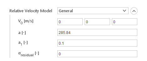
The General relative velocity model calculates dispersed diffusion velocity using the formula:
\(U_d=\frac{\rho_c}{\rho}\cdot V_0 (e^{a \alpha_d}-e^{a_1 \alpha_d})\)
where:
- \(V_0\) - drift velocity
- \(\rho_c\) - continuous phase density
- \(\rho\) - mixture density
- \(a_d\) - dispersed phase fraction
- \(a\) - model constant
- \(a_1\) - model constant
Inputs:
- \(V_0 [m/s]\) - drift velocity
- \(a [-]\) - model constant
- \(a_1 [-]\) - model constant
- \(a_{residual} [-]\) - minimum dispersed phase fraction for model to be applied
Inter Solver
The Inter family of solvers requires you to specify the surface tension between the two phases.
Inputs:
- \(\sigma [N/m]\) - surface tension between phases
Inter Mixing Solver

The Inter Mixing solver requires you to specify the surface tension and diffusion coefficient between the two phases.
Inputs:
- \(\sigma_{12} [N/m]\) - surface tension between first and second phase
- \(\sigma_{13} [N/m]\) - surface tension between first and third phase
- \(D_{23} [m^2/s]\) - diffusion coefficient between second and third phase
Inter Phase Change Solver
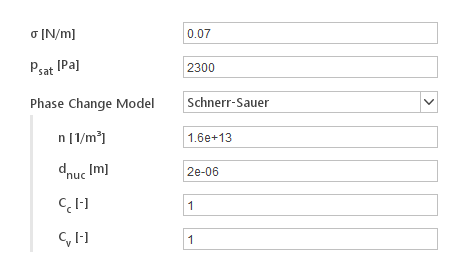
The Inter Phase Change solver is used to model phase transition due to cavitation.
Inputs:
- \(\sigma [N/m]\) - surface tension between phases
- \(p_{sat} [Pa]\) - saturation pressure
Additionally, you will have to specify a Phase Change Model .
Available phase change models:
- Schnerr-Sauer
- Merkle
- Kunz
Schnerr-Sauer Model
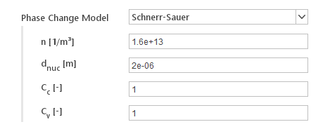
Schnerr-Sauer cavitation model.
Reference:
Schnerr, G. H., And Sauer, J.,
"Physical and Numerical Modeling of Unsteady Cavitation Dynamics",
Proc. 4th International Conference on Multiphase Flow,
New Orleans, U.S.A., 2001.
Inputs:
- \(n [1/m^3]\) - bubble number density
- \(d_{nuc} [m]\) - nucleation site diameter
- \(C_c [-]\) - condensation rate coefficient
- \(C_v [-]\) - vaporization rate coefficient
Merkle Model
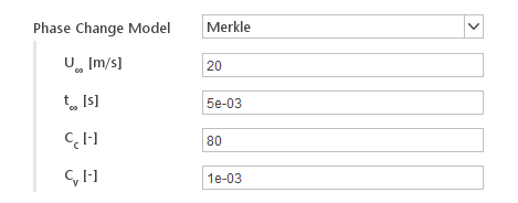
Merkle cavitation model.
Reference:
C. L. Merkle, J. Feng, and P. E. O. Buelow,
"Computational modeling of the dynamics of sheet cavitation",
in Proceedings Third International Symposium on Cavitation
Grenoble, France 1998.
Inputs:
- \(U_{\infty} [m/s]\) - characteristic velocity of the flow
- \(t_{\infty} [s]\) - characteristic time scale of the flow
- \(C_c [-]\) - condensation rate coefficient
- \(C_v [-]\) - vaporization rate coefficient
Kunz Model
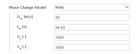
Modified version of the Kunz cavitation model, where the condensation term is switched off when the pressure is less than the saturation pressure.
Reference:
Kunz, R.F., Boger, D.A., Stinebring, D.R., Chyczewski, Lindau. J.W., Gibeling, H.J., Venkateswaran, S., Govindan, T.R.,
"A Preconditioned Implicit Method for Two-Phase Flows with Application to Cavitation Prediction,"
Computers and Fluids, 29(8):849-875, 2000.
Inputs:
- \(U_{\infty} [m/s]\) - characteristic velocity of the flow
- \(t_{\infty} [s]\) - characteristic time scale of the flow
- \(C_c [-]\) - condensation rate coefficient
- \(C_v [-]\) - vaporization rate coefficient
Solvers with variable number of phases
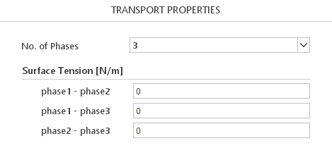
Certain solvers allow you to define the number of phases. You can do this using the No. of Phases input. Additionally for those solvers you will have to define surface tension between every pair of the phases.
Diameter Models

For multi-phase solvers that use Euler formulation, you will have to additionally define Diameter Model for the dispersed phase. Diameter model defines the granularity of the dispersed phase.
Available Diameter Models:
- Constant
- Isothermal
Constant Diameter Model

In this model diameter of the dispersed phase is fixed.
Inputs:
- \(d [-]\) - diameter
Isothermal Diameter Model

In this model, dispersed phase diameter can change due to isothermal expansion.
Inputs:
- \(d_0 [m]\) - reference diameter for the isothermal expansion
- \(p_0[Pa]\) - reference pressure for the isothermal expansion
Material Database
Instead of specify each of the material properties by hand, you can load them from the material database. When you click the Material Database button, the Material Selection dialog will be displayed.
Material Selection
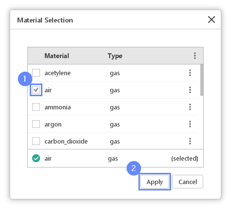
In the Material Selection dialog you can apply material properties of one of the available.
To apply material properties:
1 Selected a checkbox next to material name.
2 Click Apply to load properties from selected materal.