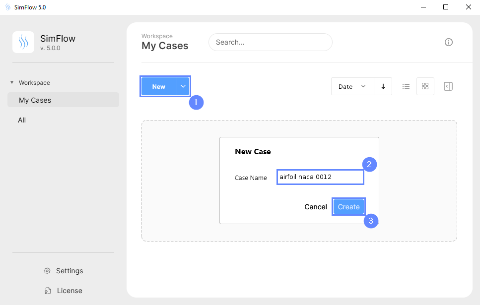
3. Create Case
Open SimFlow and create a new case named airfoil naca 0012
- Click New
- Provide name airfoil naca 0012
- Click Create to open a new case
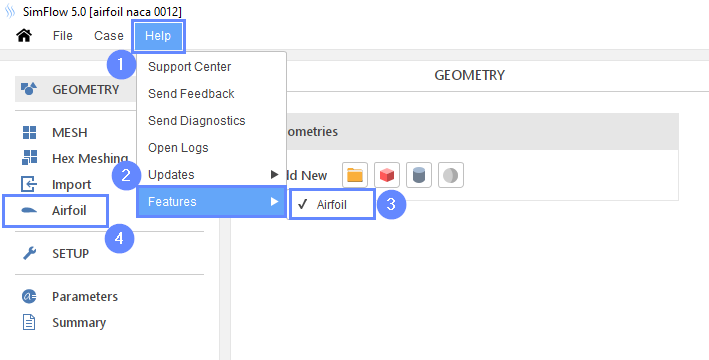
4. Enable Airfoil Feature
We need to enable the Airfoil feature in SimFlow from the menu bar:
- Expand the Help menu
- Select Features
- Enable the Airfoil feature
- Airfoil panel should appear on the left panel list
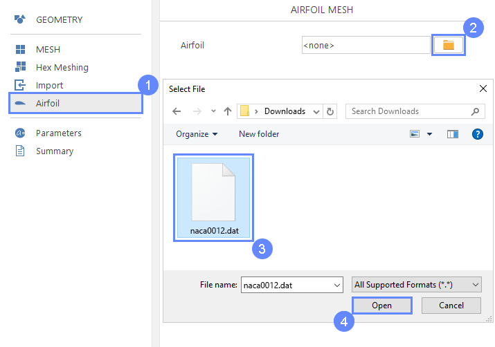
5. Import Geometry
Firstly we need to Download GeometryNaca0012
- Go to Airfoil panel
- Click Import Geometry
- Select geometry file naca0012.dat
- Click Open
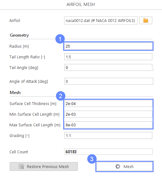
6. Airfoil Meshing
- Set Radius [m] to 25 meters
- Set the following parameters accordingly
Surface Cell Thickness \({\sf [m]}\)2e-04
Min Surface Cell Length \({\sf [m]}\)2e-03
Max Surface Cell Length \({\sf [m]}\)8e-03 - Click Mesh to start the meshing process
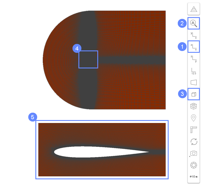
7. Mesh
After creating a mesh, it will appear in the 3D window.
- Click XZ View
- Click Fit View to zoom the mesh
- Change view projection from Perspective to Parallel
- Zoom in the middle section of the mesh by using scroll mouse button
- If you zoom in enough, airfoil shape should appear
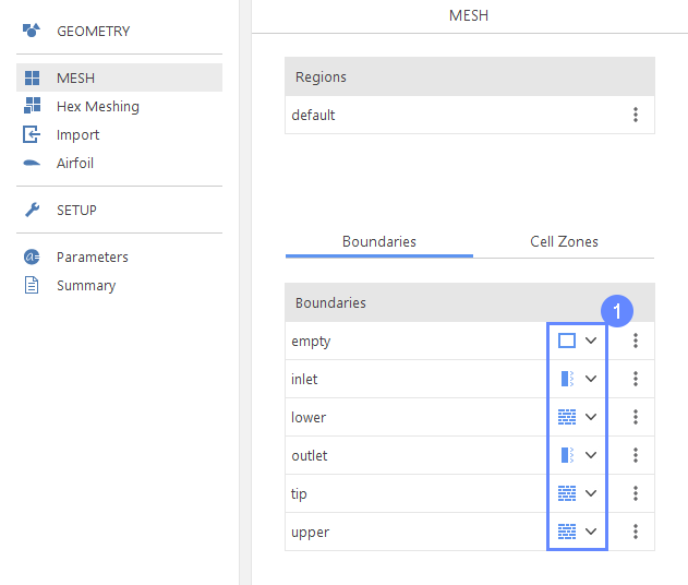
8. Inspect Mesh Boundaries
Now we will check if the boundaries are set properly.
- Inspect boundaries
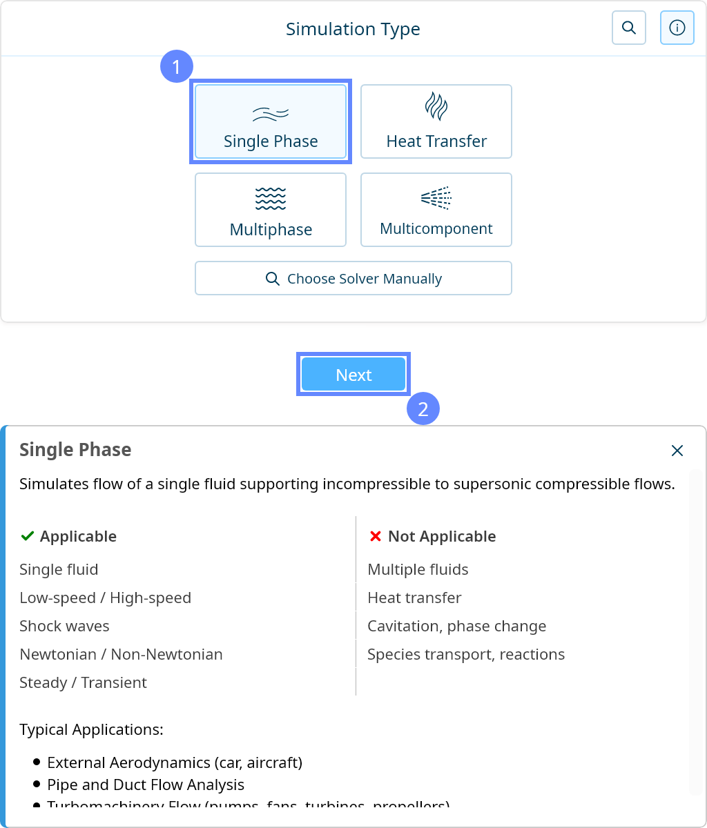
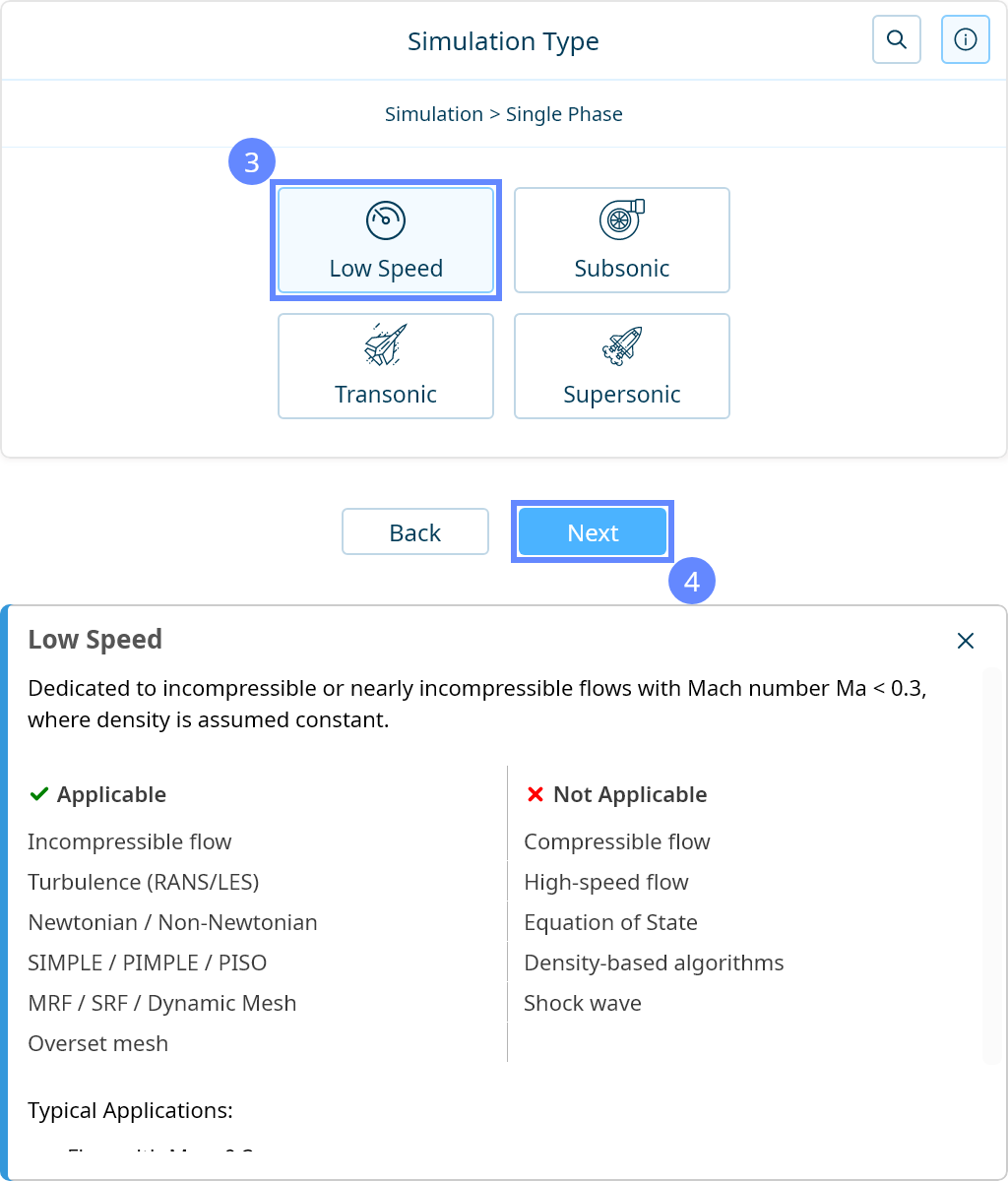
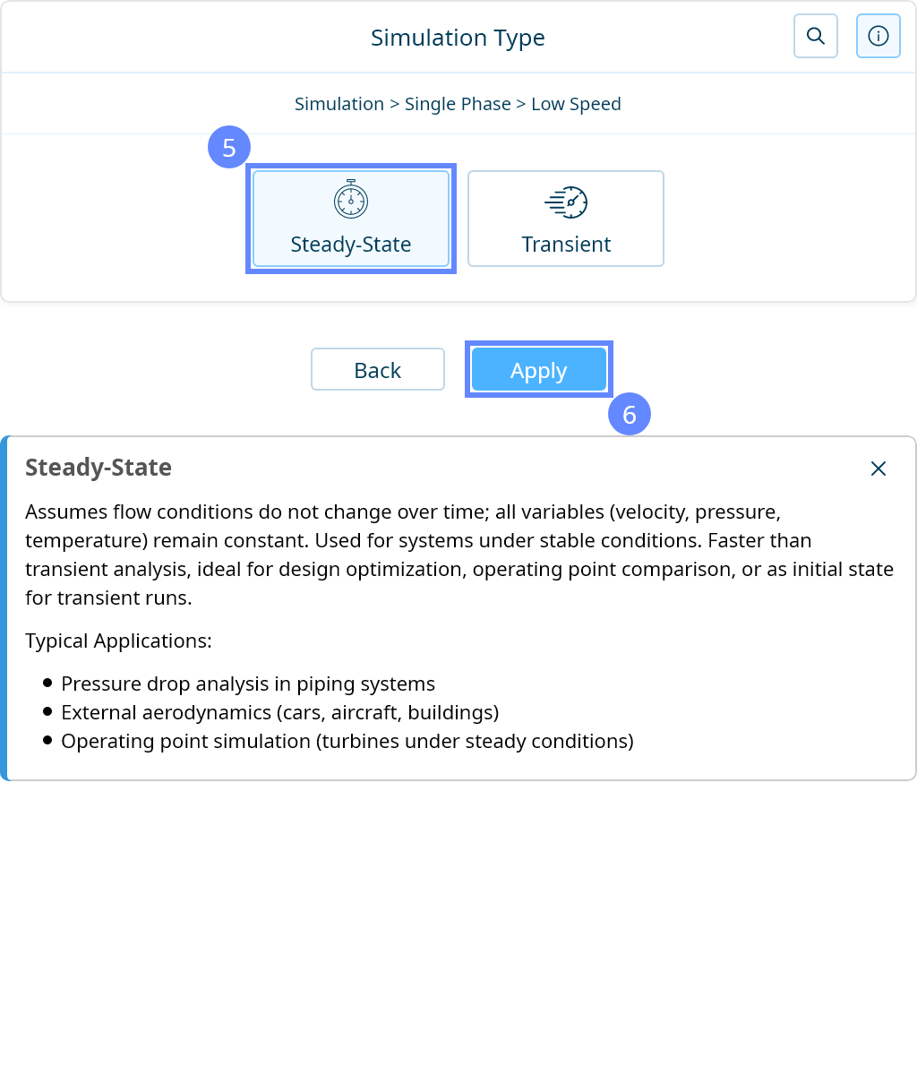
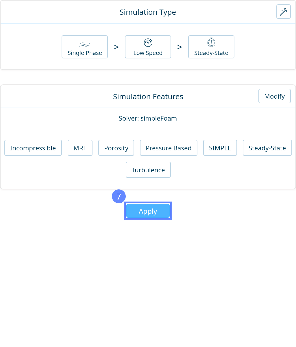
9. Simulation Type
We want to analyze the airflow around the airfoil. For this purpose, we will use a single-phase, steady-state simulation of incompressible turbulent flow.

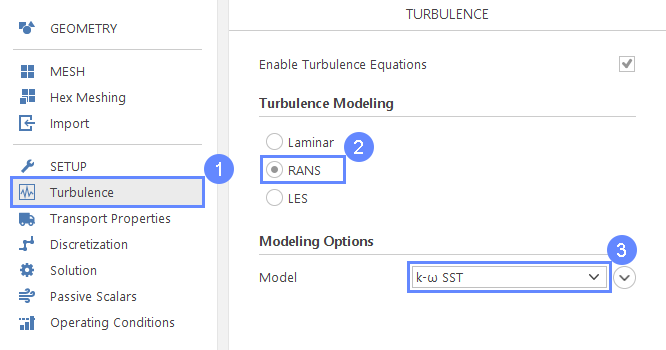
10. Turbulence
We are going to use the standard \(k-\omega \; SST\) model to handle turbulence. This model gives very good agreement with experimental data and is commonly used for aerodynamics applications.
- Go to Turbulence panel
- Select RANS modeling
- Select \(k-\omega \; SST\) model
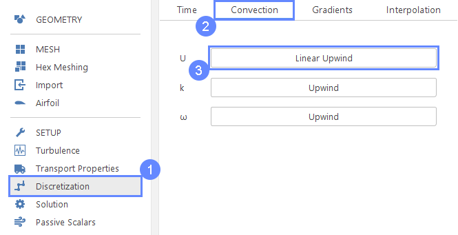
11. Dicretization - Convection
- Go to Discretization panel
- Go to Convection tab
- Select Linear Upwind for U (Velocity) parameter
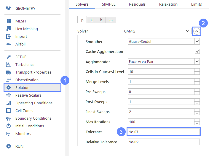
12. Solution - Solvers (Pressure)
The calculations will be run until Residuals will drop down under 10 −6 . This criterion will guarantee high accuracy and will require more iteration. To make sure that the fluid solver will be able to capture very small changes in the flow, we need to make sure that the linear solvers for fluid flow equations will also be able to operate on very slight flow changes. To do this, we will change default solver tolerances.
- Go to Solution panel
- Expand list of options
- Set Tolerance to 1e-07
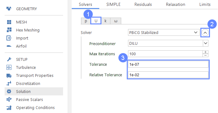
13. Solution - Solvers (Velocity)
- Go to U (Velocity) tab
- Expand list of options
- Set following parameters accordingly
Tolerance1e-07
Relative Tolerance1e-02
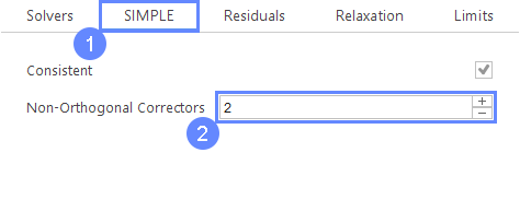
14. Solution - SIMPLE
- Go to SIMPLE tab
- Set Non-Orthogonal Corrections to 2
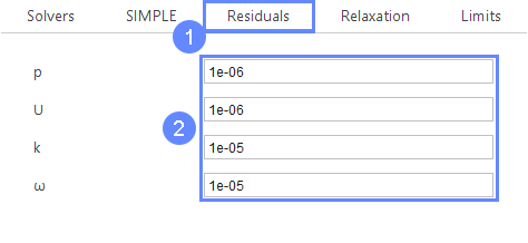
15. Solution - Residuals
- Go to Residuals tab
- Set following parameters accordingly
p1e-06
U1e-06
k1e-05
\(\omega\)1e-05
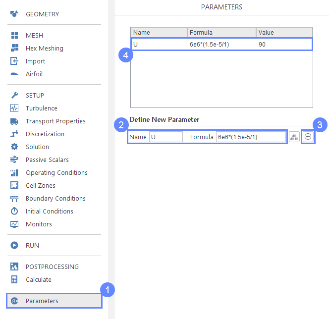
16. Parameter - U (Velocity)
It is handy to parameterize velocity value to be easily accessible in the further setup. To be able to compare the results with test results we should assume \(Re=6000000\). Based on the air viscosity \(\nu = 1.5 \cdot 10^{-5} \; m^2/s \) and chord \(c\approx 1 \;m\) we calculate the velocity from the equation: \(V=Re \cdot \frac{\nu}{c}\)
- Go to Parameters panel
- Define the name and formula of the new parameter
NameU
Formula6e6*(1.5e-5/1) - Click Create Parameter
- The newly created parameter will be shown in the parameters list
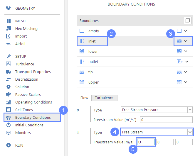
17. Boundary Conditions - Inlet (Flow)
- Go to Boundary Conditions panel
- Select inlet boudary
- Change boundary character to Free Stream
- Set to velocity type to Free Stream
- Now we can use parameter U defined earlier
Freestream Value \({\sf [m/s]}\)U00
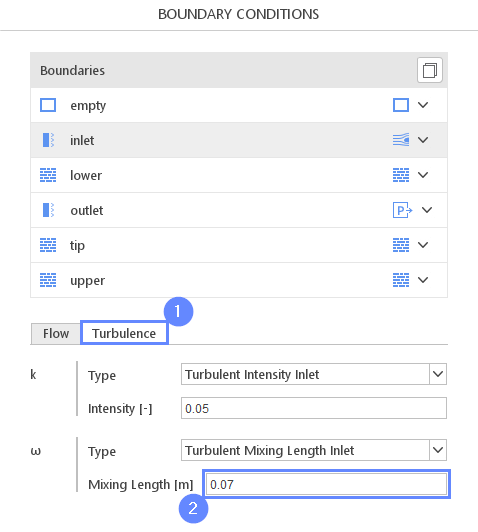
18. Boundary Conditions - Inlet (Turbulence)
- Go to Turbulence tab
- Set Mixing Length \({\sf [m]}\)0.07
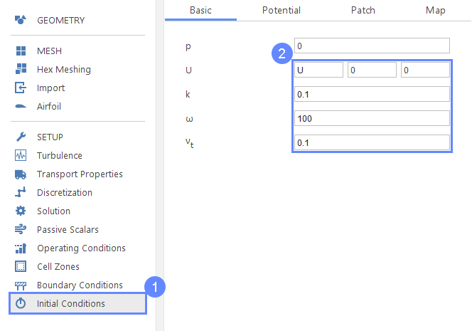
19. Initial Conditions - Basic
- Go to Initial Conditions panel
- Set following initial conditions accordingly
UU00
k0.1
\(\omega\)100
\(\nu_t\)0.1
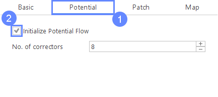
20. Initial Conditions - Potential
We will use the "Potential" initialization feature. This utility solves pseudo potential flow prior to actual calculations. This will give a better initial guess for velocity and pressure fields.
- Go to Potential tab
- Check Initialize Potential Flow
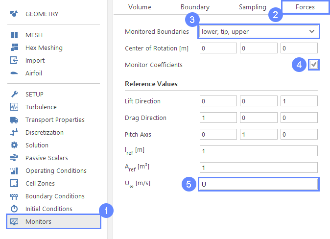
21. Monitors - Forces
- Go to the Monitors panel
- Go to the Forces tab
- For Monitor Boundaries select lower tip upper
- Check Monitor Coefficients
- Define free stram velocity accordingly
\(U_\infty\) \({\sf [m/s]}\)U
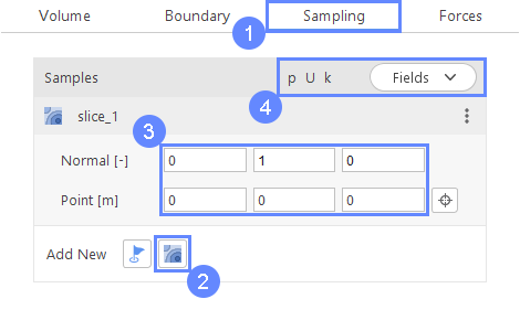
22. Monitors - Create Slice
Additionally to observing force coefficients, we will display intermediate results on a section plane.
- Go to Sampling tab
- Add new Slice
- Set the follwing parameters accordingly
Normal \({\sf [-]}\)010
Point \({\sf [m]}\)000 - Expand Fields menu. Choose p U k (pressure, velocity and turbulent kinetic energy) to be sampled on the section plane.
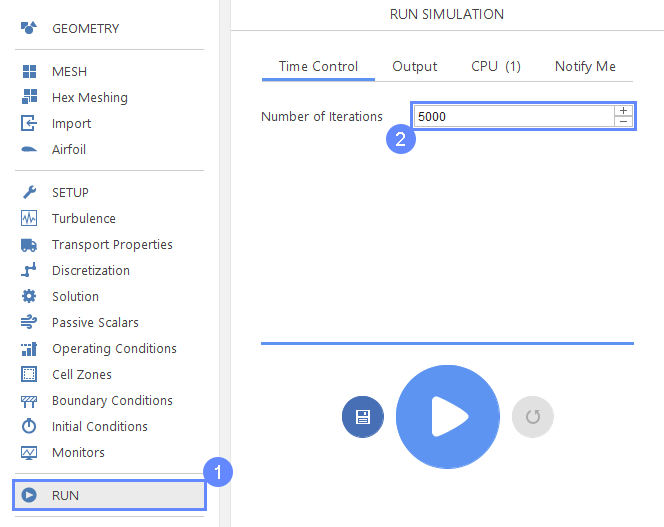
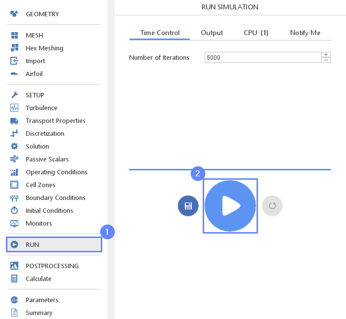
23. Run - Time Control
- Go to Run panel
- Set Number of Iterations to 5000
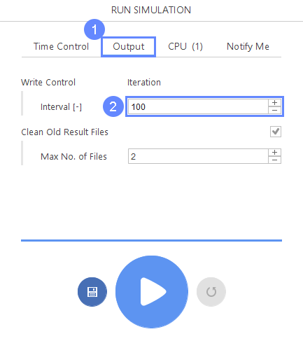
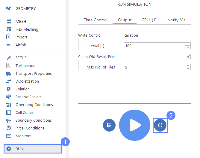
24. Run - Output
- Go to Output tab
- Set Interval [-] to 100
This controls when results are written to the hard drive. When slices are enabled this also applies to them. Each new result will be displayed at a specified interval.
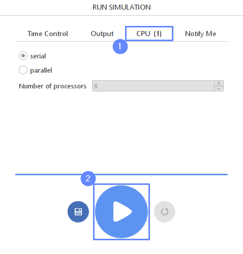
25. Run - CPU
To speed up the calculation process, take advantage of parallel computing and increase the number of CPUs based on your PC’s capability. The free version allows you to use only one processor (serial mode). To get the full version, you can use the contact form to Request 30-day Trial
Estimated computation time for serial mode: 25 minutes
- Switch to CPU tab
- Click Run Simulation button
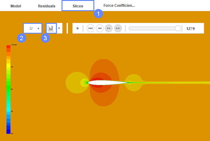
26. Slice - View Velocity field
- Change tab to Slices
- Choose U (Velocity) field
- Click Adjust range to data adjust color range to actually displayed data
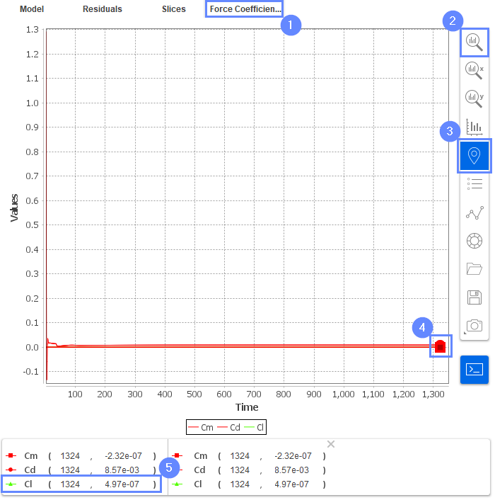
27. Results - Force Coefficients
- Change tab to Force Coefficients
- Click Fit Axes
- Select Lookup Data
- Choose the last point from the chart
- Read the Lift coefficient
28. Reset Simulation
If you want to change the angle of the attack, you should first reset the simulation in the run panel.
- Go to Run Panel
- Reset Simulation
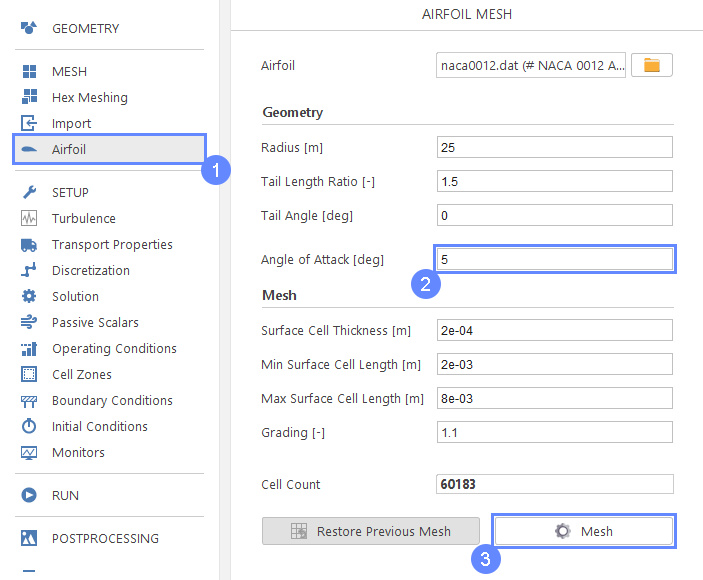
29. Change Angle of Attack
In the Airfoil panel, we can now remesh the Airfoil change angle of attack. And then rerun the simulation.
- Go to Airfoil panel
- Change the Angle of attack for the desired value for example
Angle of Attack \({\sf [deg]}\)5 - Click Mesh button
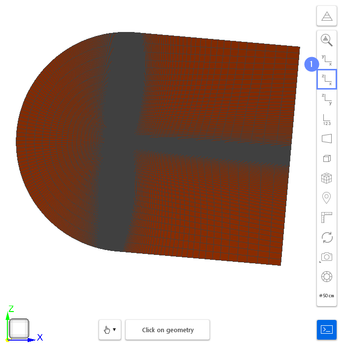
30. Mesh - Second Case
After creating a mesh, it will appear in the 3D window.
- Click XZ View
31. Run Second Simulation
- Go to Run panel
- Click Run Simulation button
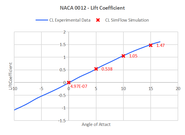
32. Results Comparison With Experimental Data
You might repeat the above operations for different angles of attack, e.g: 5, 10 and 15 degrees. Next comparing them with the experimental data (NASA Langley, 1988) you should be able to obtain the following results.