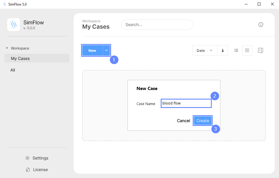
3. Create Case
Open SimFlow and create a new case named blood flow
- Click New
- Provide name blood flow
- Click Create to open a new case
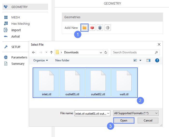
4. Import Geometry
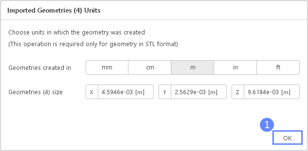
5. Imported Geometry Units
The STL format does not contain the unit information which are defined during the geometry export. Therefore, you must manually specify the correct unit after import. If we do not know the exported unit, we can estimate it based on the total size of imported geometries. The size is displayed next to Geometry size label. In our case, the default unit meter is correct.
- To confirm default unit meter, press OK
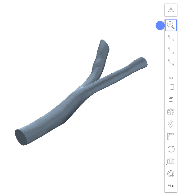
6. Geometry - Blood Vessel
After importing geometry it will appear in the 3D window.
- Click Fit View to zoom in on the geometry
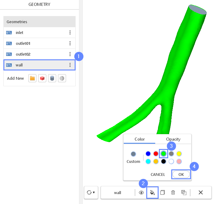
7. Display Geometry - Blood Vessel
We will change the color of the wall to distinguish it from the other geometries.
- Select the wall from geometry list or hold CTRL key and click on the wall face
- Click Change Object Display Properties
- Select
greencolor - Approve by clicking OK
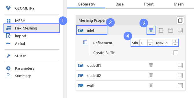
8. Meshing Parameters - Inlet
In the Hex Meshing panel, we will change meshing properties associated with geometry objects. We want to apply the same settings to all geometries. We will set the parameters for the first surface and copy the configuration to the remaining geometries.
- Go to Hex Meshing panel
- Select the inlet component
- Enable Mesh Geometry
- Set Refinement to Min 1 Max 1
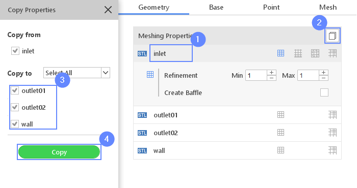
9. Meshing Parameters - Copy
We want to apply the same settings to all geometries. We will copy the configuration from the inlet to the remaining geometries.
- Select the inlet
- Click Copy Meshing Properties
- Select all the remaining faces as a target outlet01 outlet02 wall
- Click Copy
10. Base Mesh - Domain
Under the Base tab we will define the domain of the background mesh.
- Go to Base tab
- Click on Autosize
- Define the number of divisions
Division6034125
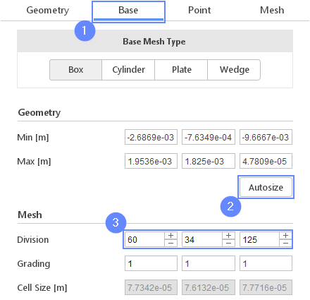
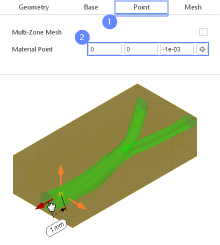
11. Material Point
Material Point tells the meshing algorithm on which side of the geometry the mesh is to be retained. Since we are considering flow inside the blood vessel we need to place the material point inside the geometry.
- Go to Point tab
- Specify location inside blood vessel geometry
Material Point00-1e-03
You can specify the point location from the 3D view. Hold the CTRL key and drag the arrows to the destination.
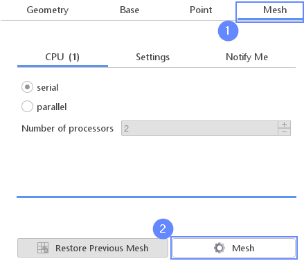
12. Start Meshing
Everything is now set up for meshing
- Go to Mesh tab
- Press Mesh button to start meshing process
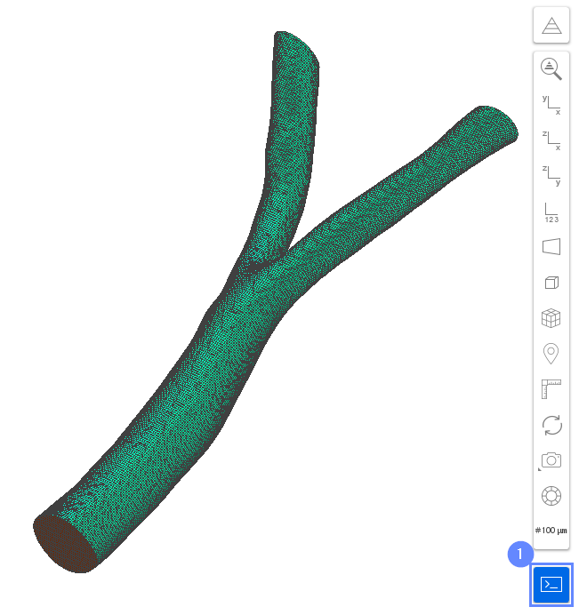
13. Mesh
After the meshing process, the mesh will appear in the graphics window. Use the scroll wheel in your mouse to zoom into the model.
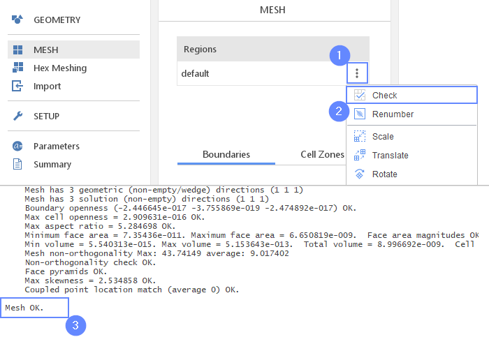
14. Check Mesh
Check the mesh quality and statistics.
- Expand the Options list next to default region
- Select Check option
- Checks summary will be displayed on the command window. It also shows checking criteria.
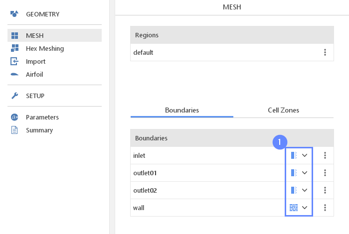
15. Mesh - Boundaries
- Set the following boundaries types accordingly
inlet Patch
outlet01 Patch
outlet02 Patch
wall Wall
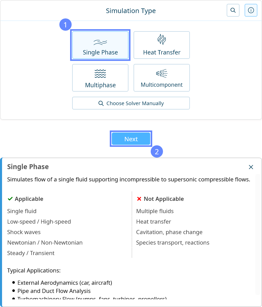
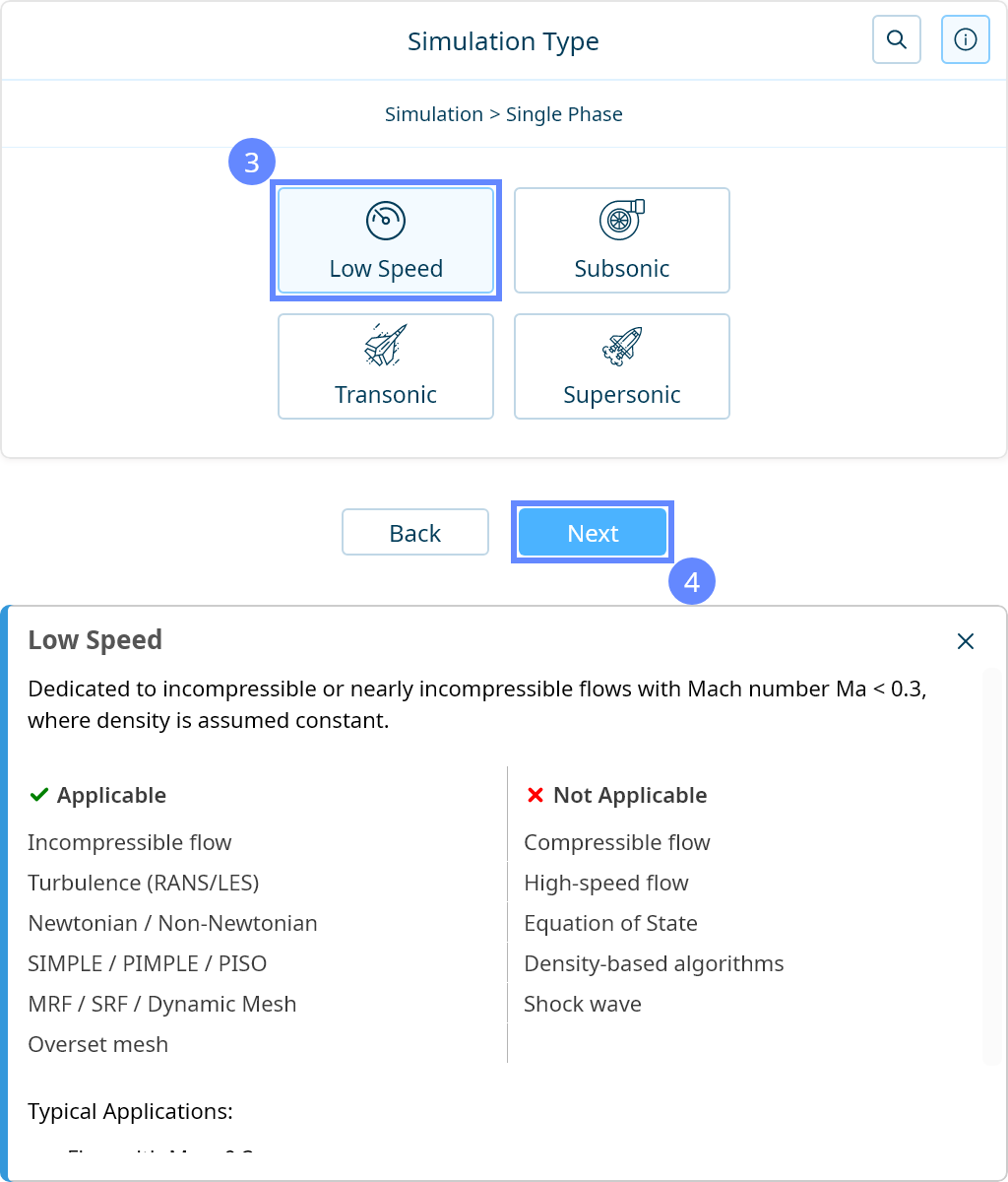
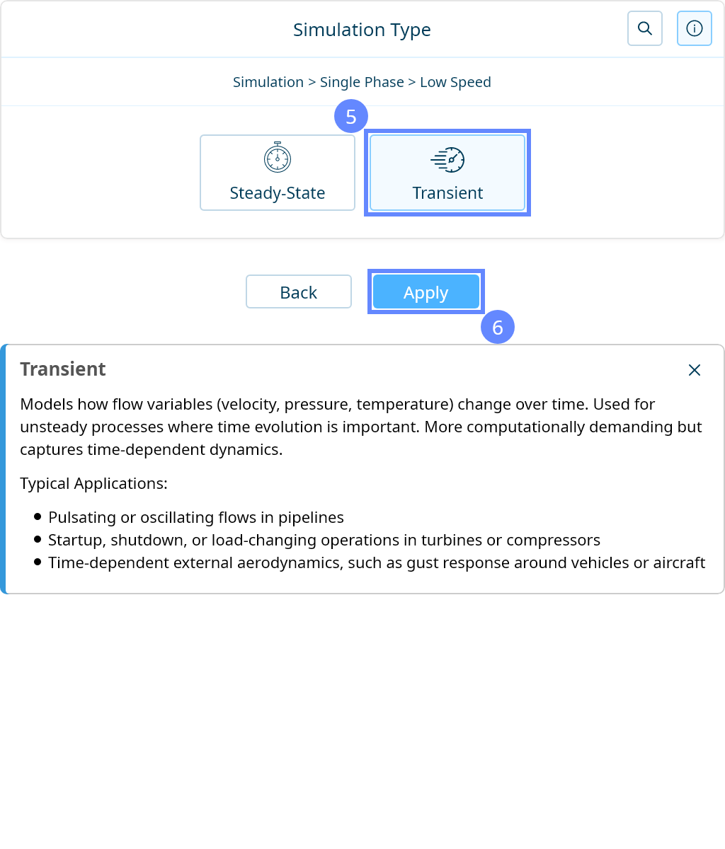
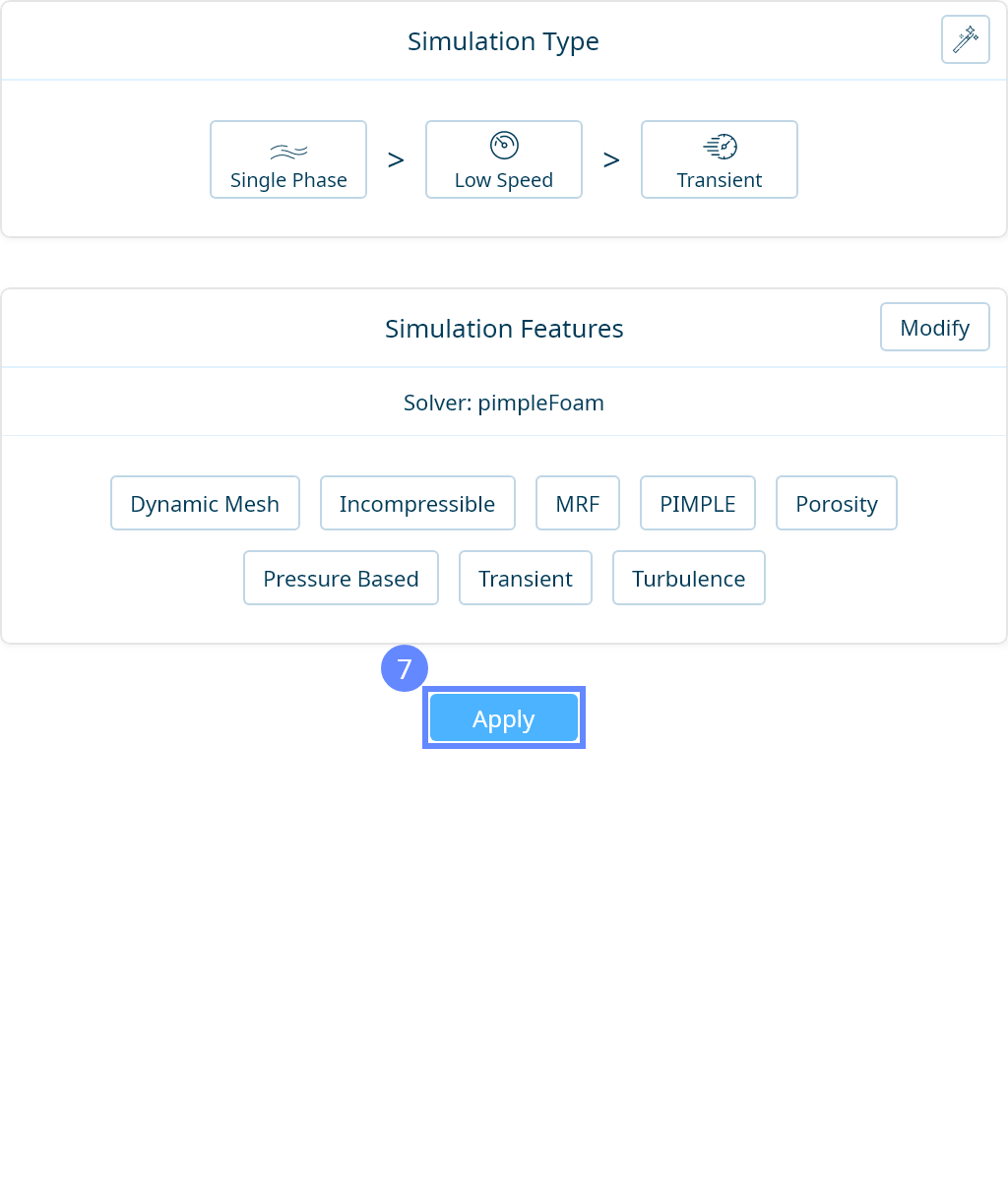
16. Simulation Type
We want to analyze the transient flow of a non-Newtonian fluid to model the blood flow. For this purpose, we will use a single-phase, incompressible flow simulation.

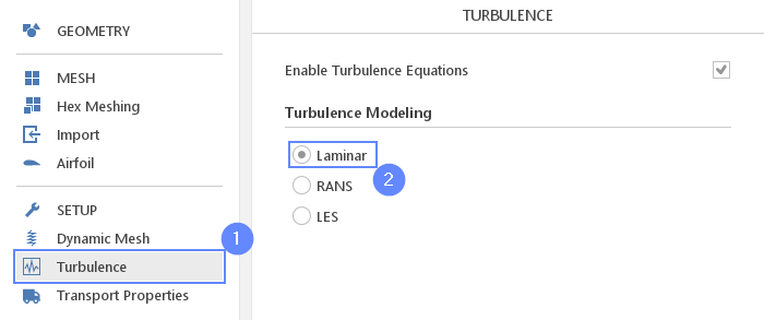
17. Turbulence
Due to the small diameter of the vessel and high viscosity of the fluid, it can be assumed that the flow remains laminar.
- Go to Turbulence panel
- Make sure the Laminar model is selected
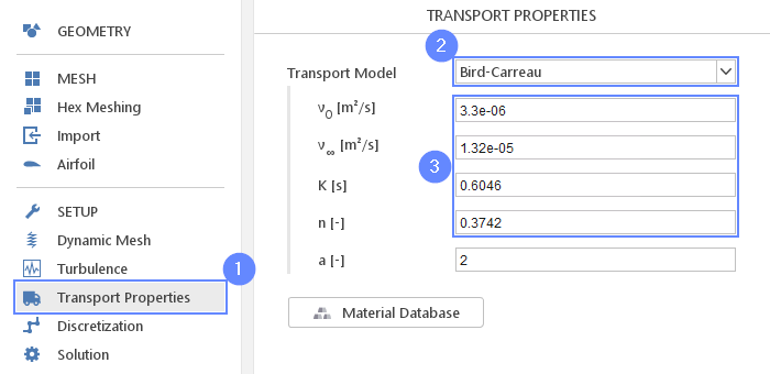
18. Transport Properties
For the demonstration purpose, we will model the blood as non-newtonian fluid using the Bird-Carreu model. We will operate on quantities divided by density and we do not need to specify the density. However, we have to take this fact into account during postprocessing.
- Go to Transport Properties panel
- Change Transport Model to Bird-Carreau
- Set the parameters accordingly
\(\nu_0\) \({\sf [\frac{m^2}{s}]}\)3.3e-06
\(\nu_{\infty}\) \({\sf [\frac{m^2}{s}]}\)1.32e-05
\(K\) \({\sf [s]}\)0.6046
\(n\) \({\sf [-]}\)0.3742
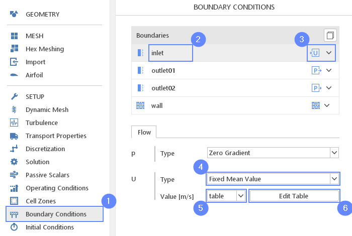
19. Boundary Conditions - Inlet (I)
The flow in the blood vessels is oscillatory in time. We will define the inlet velocity using the time history of one oscillation period. To do so we will use a table input option. The rest of the boundaries conditions we will leave as default.
- Go to Boundary Conditions panel
- Select the inlet boundary
- Set the Velocity Inlet character
- Change the Type of the velocity to the Fixed Mean Value
- Change the Value [m/s] to the table
- Click on Edit Table
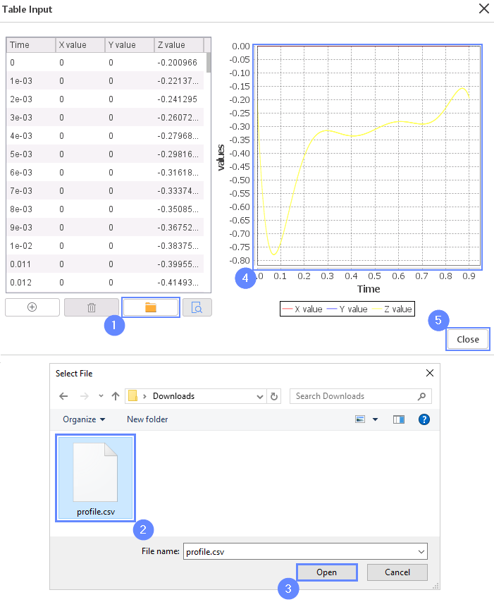
20. Boundary Conditions - Inlet (II)
We will use a predefined velocity profile from the external file.
We need to Download Velocity Profileprofile.csv and import it to the Simflow.
- Click on Load Data From File
- Select the profile.csv file
- Press OK
- Loaded data will be presented on the chart
- Press Close
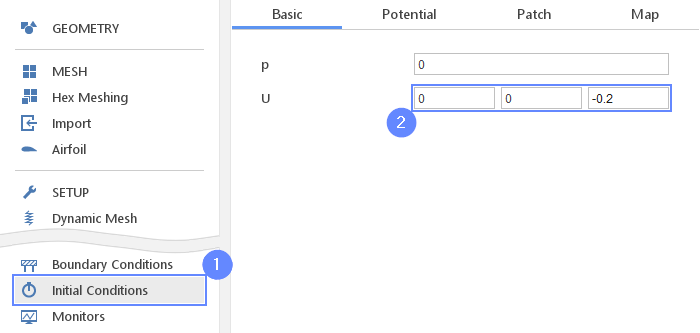
21. Initial Conditions
Before we start simulation we need to define the flow state at the time zero. We will specify a constant velocity equal to ` 0.2 m/s ` which corresponds to the initial inlet velocity.
- Go to Initial Conditions panel
- Set the initial velocity
U00-0.2
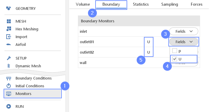
22. Monitors - Boundary
We would like to monitor flow velocity at the outlet boundaries. The results can be later on used to calculate the volumetric and mass flow rates for each outlet.
- Go to Monitors panel
- Switch to Boundary tab
- Expand Fields for the outlet01
- Select the velocity field U
- Repeat this step for the outlet02 boundary.
Selected fields will be visible next to the boundary names.
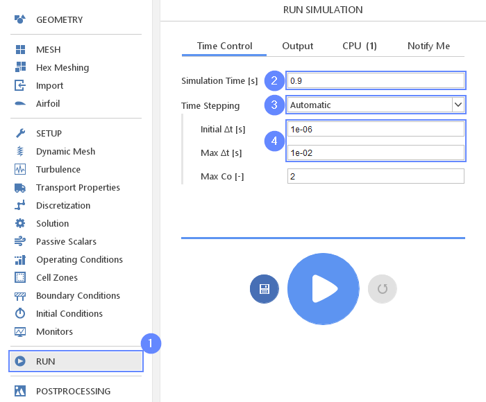
23. Run - Time Control
We will set the time of simulation to match the inlet velocity time range. We also want the solver to automatically determine the proper time step. This should lead to good stability and potentially reduce simulation time.
- Go to RUN panel
- Set the Simulation Time [s] to 0.9
- Change Time Stepping \(\Delta t[s]\) to Automatic
- Set initial and maximum time step (solver will start computation with initial value and adjust it in the next iterations not exceeding the maximum value)
Initial \(\Delta t\) \({\sf [s]}\)1e-06
Max \(\Delta t\) \({\sf [s]}\)1e-02
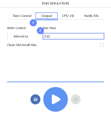
24. Run - Output
We can control how often results should be saved on the hard drive. We will write the results at the interval of ` 0.02 ` seconds. Note, that only saved data will be available during postprocessing.
- Switch to Output tab
- Set the Interval [s] to 0.02
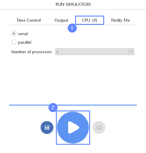
25. Run - CPU
To speed up the calculation process, take advantage of parallel computing and increase the number of CPUs based on your PC’s capability. The free version allows you to use only one processor (serial mode). To get the full version, you can use the contact form to Request 30-day Trial
Estimated computation time for serial mode: 1,5 hours
- Switch to CPU tab
- Click Run Simulation button
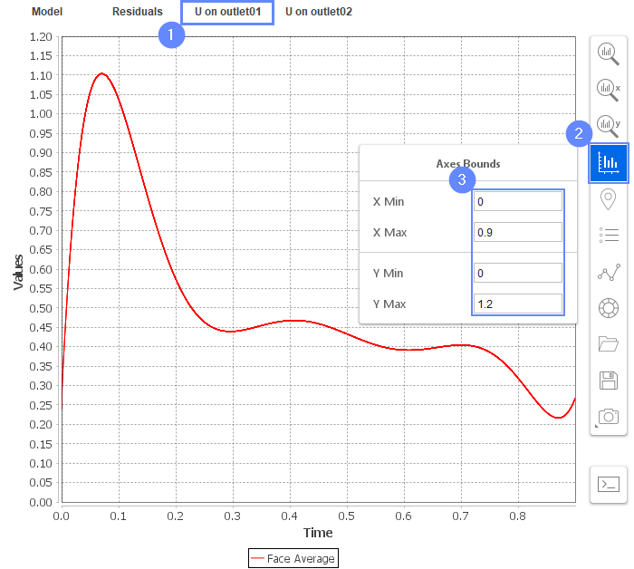
26. Results - Outlet Velocity
Outlet boundary monitors are ploted on the charts next to Residual tab.
- Switch to U on outlet01 tab
- Click Adjust Axes
- Set the range for X and Y axis:
X Min0
X Max0.9
Y Min0
Y Max1.2
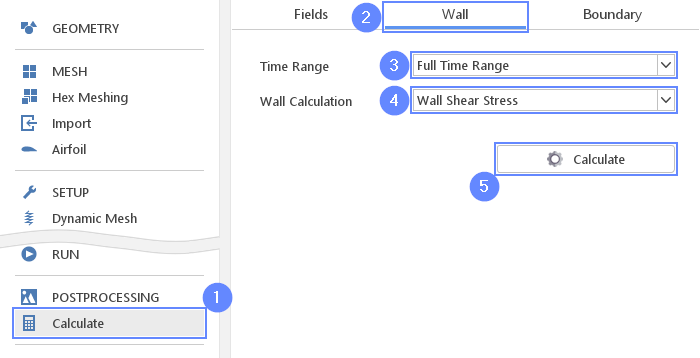
27. Calculate Wall Shear Stress
Calculations are finished, but before we start postprocessing, we will calculate wall shear stress (WSS). It can be calculated as the multiplication of dynamic viscosity and velocity gradient next to the wall. WSS is a characteristic value in medicine, used for circulatory system disease identification. Too low values are the indicators of atherosclerosis while the large WSS leads to the thickening of the vessel wall and increasing its diameter. This occurs when one vessel splits into two like in our example.
- Go to Calculate panel
- Switch to Wall tab
- Set the Time Range to Full Time Range
- Set the Wall Calculation to Wall Shear Stress
- Click on Calculate
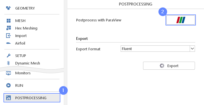
28. Postprocessing - ParaView
After computations are finished we can do complex visualization of our results with ParaView.
- Go to POSTPROCESSING panel
- Click on Run ParaView
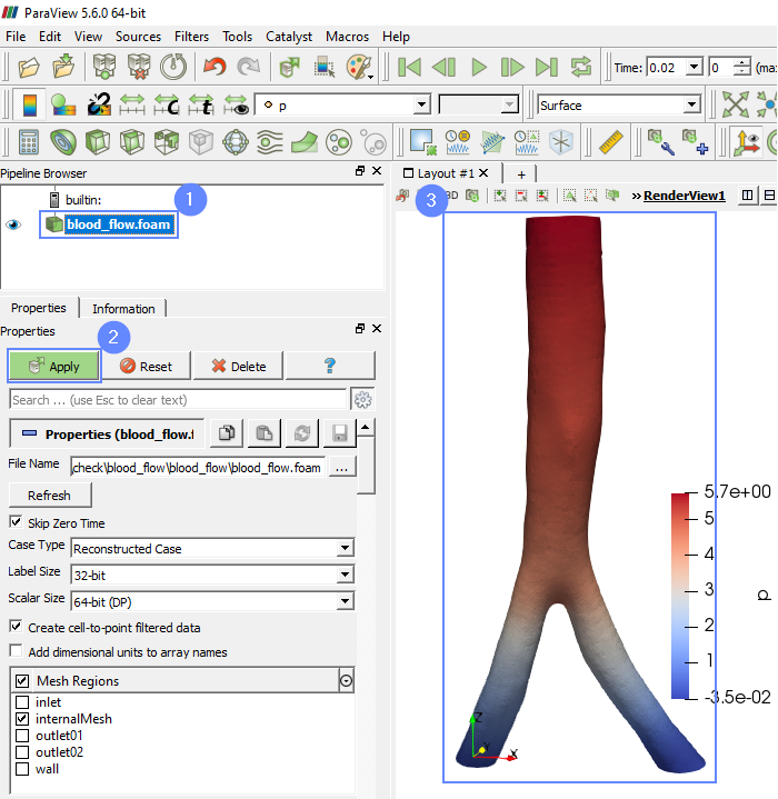
29. ParaView - Load Results (I)
Load the results into the program.
- Select blood_flow.foam
- Click Apply to load results into ParaView
- After loading results they will be shown in the 3D graphic window
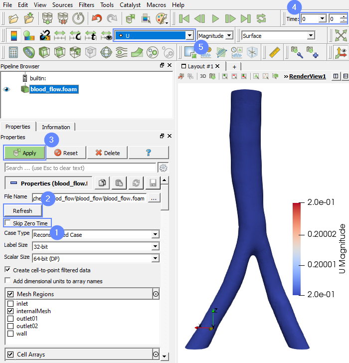
30. ParaView - Load Results (II)
ParaView skips the initial time step by default, therefore we need to add the zero time to simulation.
- Uncheck Skip Zero Time
- Click Refresh
- Click Apply
- Set the time or time step to 0
- Select the velocity U from the list
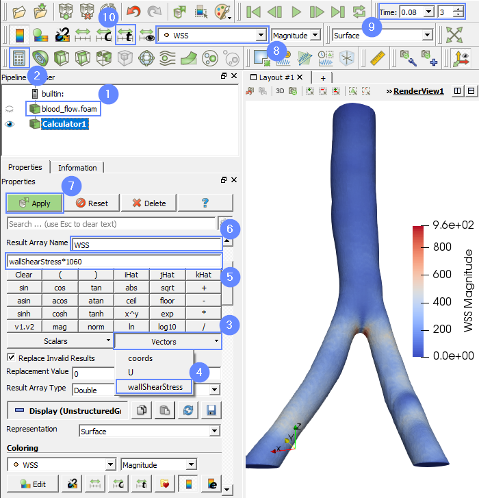
31. ParaView - WSS
To get the true value of the wall shear stress we need to multiply SimFlow results by the density. Please remember that for the sake of this tutorial we have created coarse mesh. We also model the vessel as rigid walls, whereas in reality, it’s hyper-elastic. Nevertheless, still we can identify the regions of extremely high and low wall shear stresses.
- Select blood_flow.foam
- Click Calculator
- Expand the vector list in calculator
- Select wallShearStress
- Selected vector appears in equation. Now we will multiply vector by the blood density 1060
- Set the ressult name to WSS
- Click Apply
- Select the wall shear stress WSS from the list
- Play with an animation buttons to track the results of analysis
- Click on Rescale to data range over all timesteps
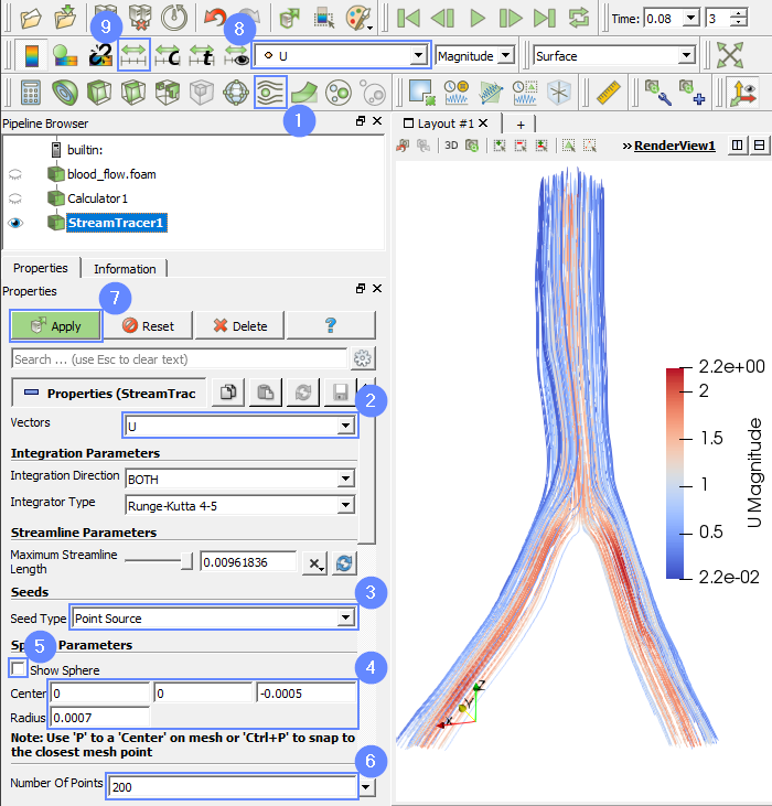
32. ParaView - Streamline (I)
Finally, we can take a look at streamlines.
- Select Stream Tracer from top menu
- Select velocity U from the vectors list
- Change Seed Type to Point Source
- Type the center coordinate and radius of the sphere:
Center00-0.0005
Radius0.0007 - Uncheck the Show Sphere
- Increase the number of points to 200
- Click Apply
- Select the velocity U from the list
- Click on Rescale to Data Range
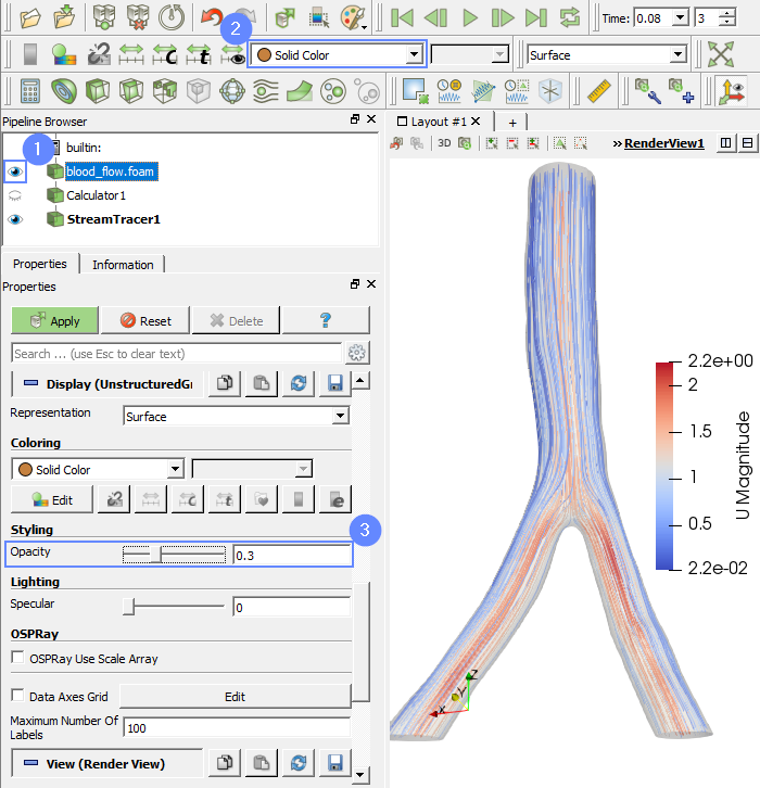
33. ParaView - Streamline (II)
To show the geometry together with the streamlines we will follow these steps:
- Click on the eye next to blood_flow.foam
- Select Solid Color from the list
- Change the opacity to 0.3