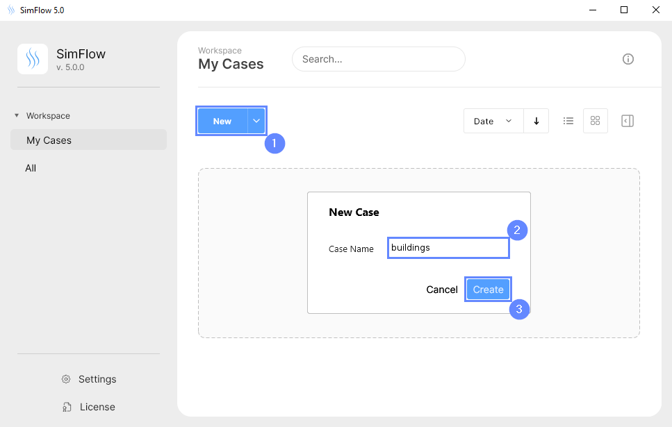
3. Create Case
Open SimFlow and create a new case named buildings
- Click New
- Provide name buildings
- Click Create to open a new case
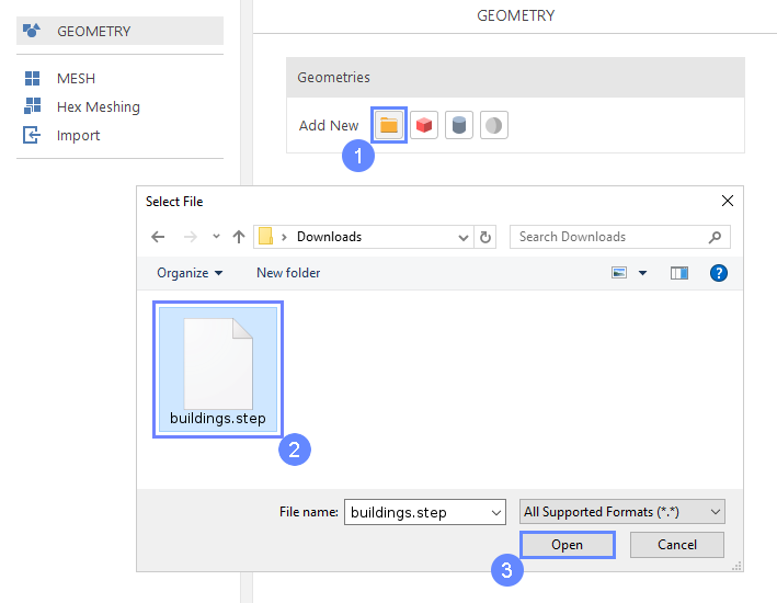
4. Import Geometry
Firstly, we need to Download GeometryBuildings
The geometry will be imported in the same units as it was exported to the STEP format.
- Click Import Geometry
- Select geometry file buildings.step
- Click Open
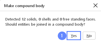
5. Import Geometry II
In some cases, the imported external geometry may contain multiple parts. SimFlow will ask you whether you want to join all geometries into a single component. If not, each part will be put into separate items.
For the purposes of this tutorial, we will combine all parts into a single geometry.
- Press Yes button
6. Geometry - Buildings
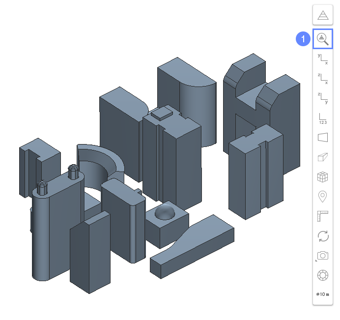
After importing geometry, it will appear in the 3D window.
- Click Fit View to zoom in on the geometry
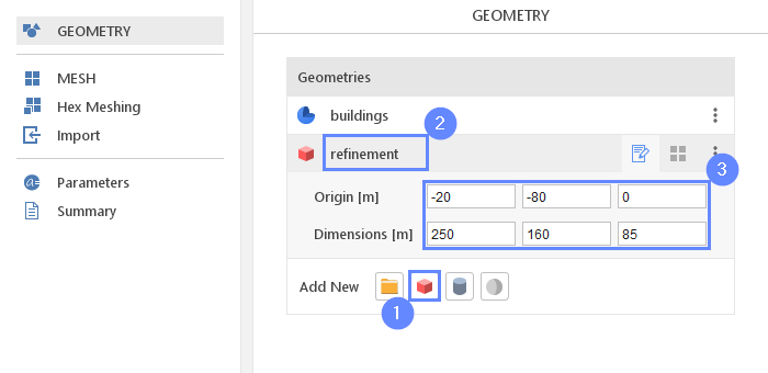
7. Create Geometry - Refinement
To be able to better resolve flow around the buildings, we will create an area with a higher mesh resolution. To do this, we will add box geometry.
- Select Create Box
- Change geometry name from box_1 to refinement
- Expand Properties
- Set the origin and box dimensions
Origin \({\sf [m]}\)-20-800
Dimensions \({\sf [m]}\)25016085
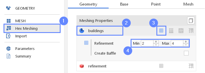
8. Meshing Properties - Buildings
After geometry is ready, we can proceed to define meshing properties. To better resolve the flow around the buildings, we want to refine mesh near the buildings geometries by specifying minimum and maximum refinement levels.
- Go to Hex Meshing panel
- Select buildings geometry
- Enable Meshing Geometry
- Set the minimum and maximum refinement level
Refinement Min 2 Max 4
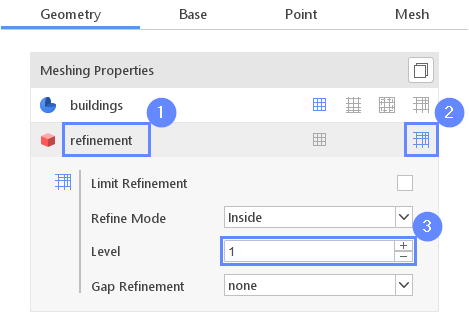
9. Meshing Parameters - Refinement
The refinement geometry should be used only for marking refinement zones. Set the proper parameters for the refinement regions.
- Click on the refinement geometry
- Enable Refine Geometry
- Set the refinement Level to 1
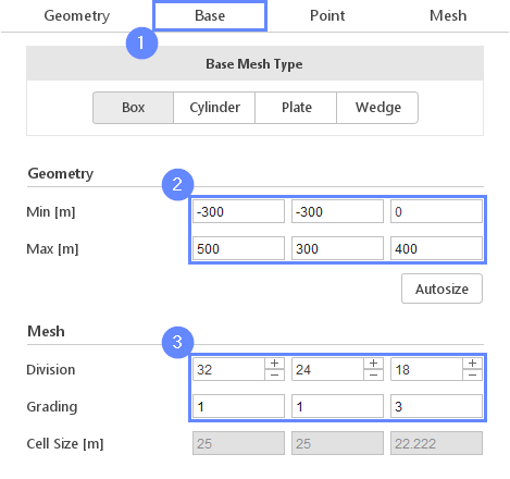
10. Base Mesh
Base Mesh is a domain mesh of our simulation from which the final mesh will be created by cutting out the geometry of the buildings.
- Go to Base tab
- Define base mesh parameters accordingly
Min \({\sf [m]}\)-300-3000
Max \({\sf [m]}\)500300400 - Set the division of the base mesh and its grading
Division322418
Grading111.07
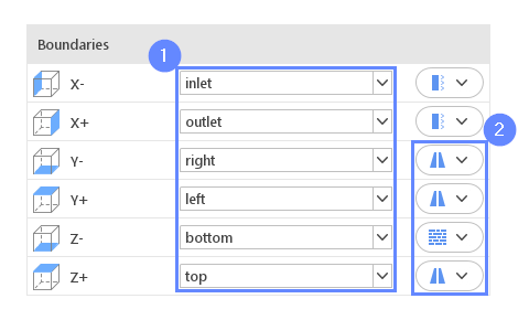
11. Base Mesh Boundaries
We need to assign individual names to each side of the base mesh in order to be later able to define different conditions on each side. To achieve simplified slip condition on side and top boundaries we will use symmetry as a boundary type.
- Define boundary names accordingly
X- inlet
X+ outlet
Y- right
Y+ left
Z- bottom
Z+ top - Define boundary types accordingly
Y- Symmetry
Y+ Symmetry
Z- Wall
Z+ Symmetry
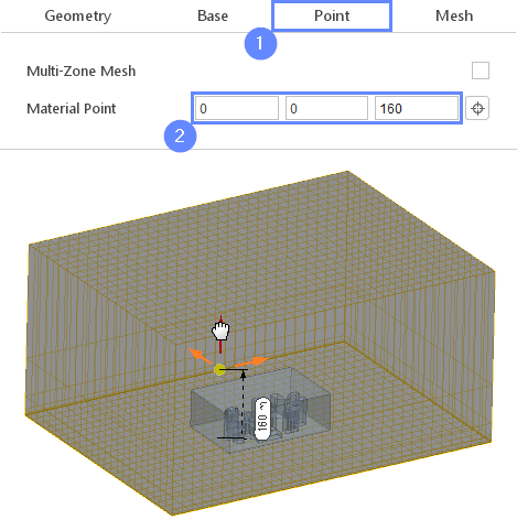
12. Material Point
Material Point tells the meshing algorithm on which side of the geometry the mesh is to be retained. We are simulating flow around the buildings so our material point needs to be located inside the base mesh but outside the buildings.
- Go to Point tab
- Specify location inside base mesh but outside buildings geometries
Material Point00160
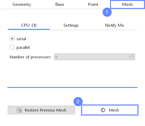
13. Start Meshing
Everything is now set up for meshing.
- Go to Mesh tab
- Press the Mesh button to start meshing process
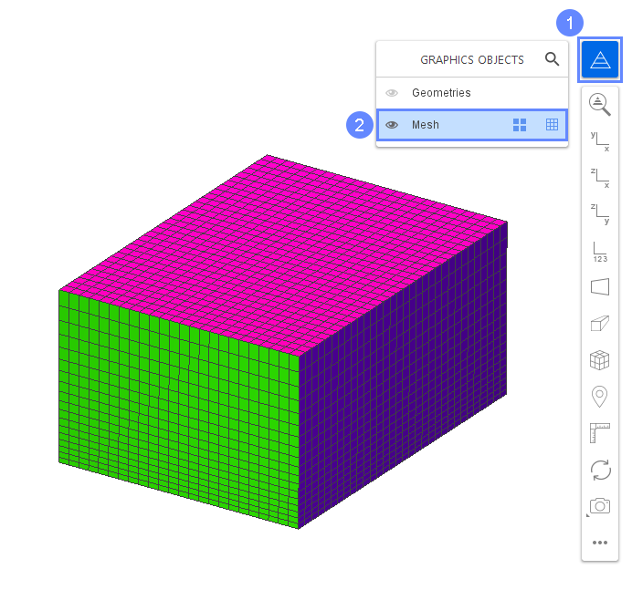
14. Mesh
The new mesh will be displayed in the graphics window. To show the mesh of the buildings we can use the Graphics Object List to hide some boundaries.
- Click Graphics Object List icon
- Select Mesh to show meshes list
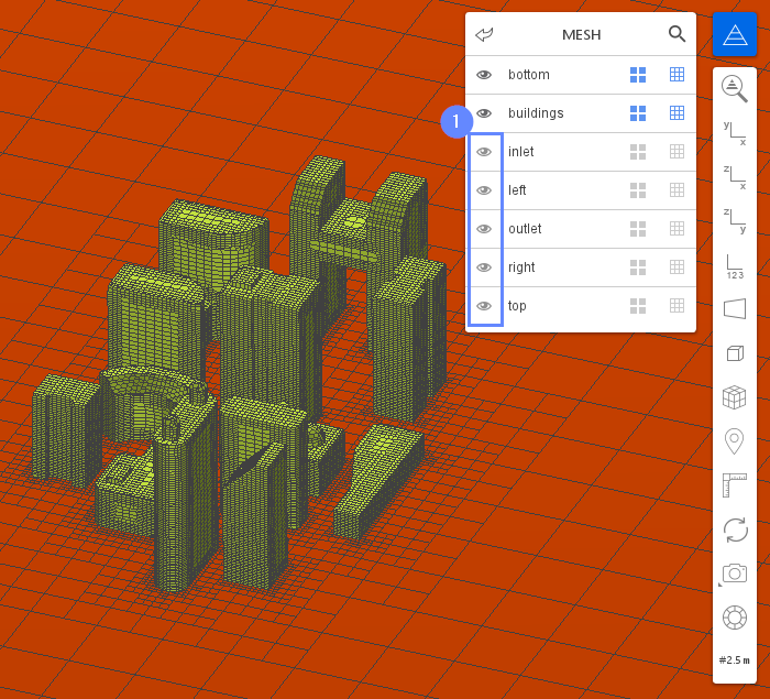
15. Mesh - Toggle Visibility
You can hide domain boundaries to inspect the mesh on the buildings.
- Hide the following objects
inlet
left
outlet
right
top
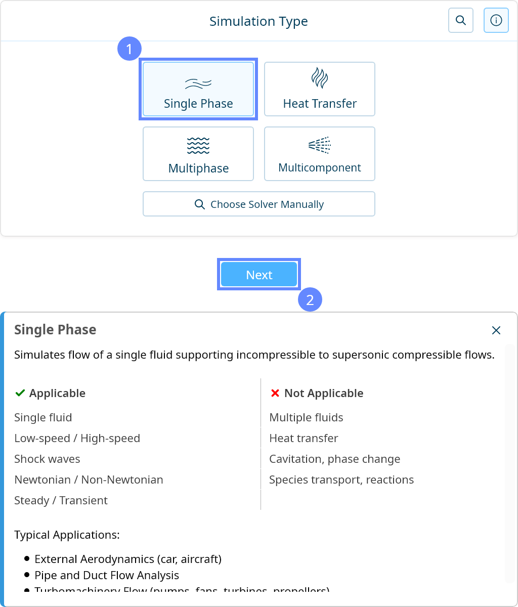
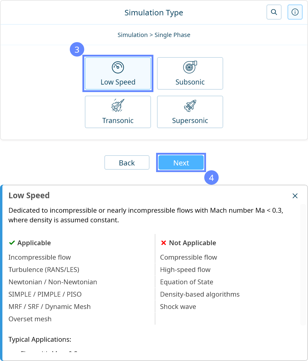
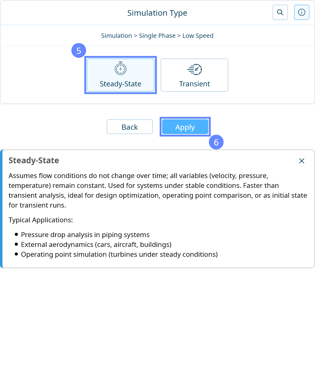
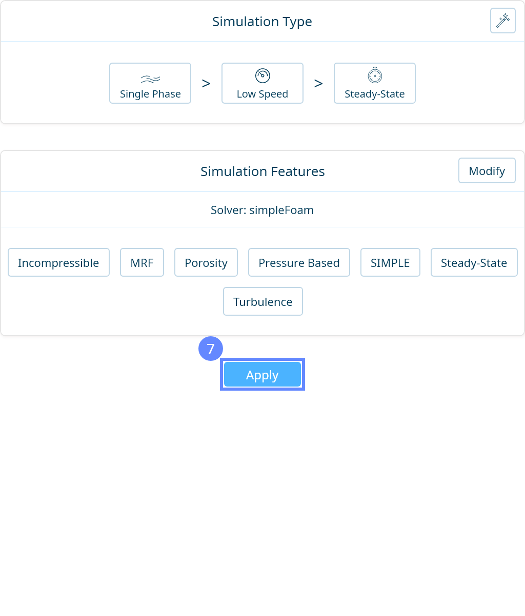
16. Simulation Type
We want to analyze the airflow around buildings. For this purpose, we will use a single-phase, steady-state simulation of incompressible turbulent flow.

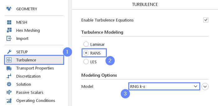
17. Turbulence
We are going to use the \(RNG \; k{-}\epsilon\) model to handle turbulence.
- Go to Turbulence panel
- Select turbulence model
Turbulence Modelling RANS - Change default turbulence model
Model \(RNG \; k{-}\epsilon\)
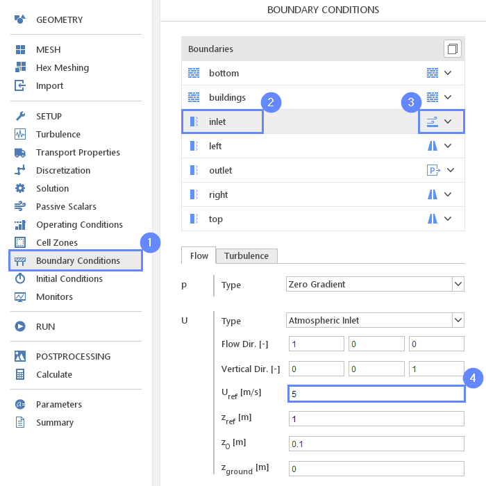
18. Boundary Conditions - Inlet
On the inlet boundary, we are going to apply Atmospheric Inlet boundary condition. It is dedicated condition for atmospheric airflow. The Atmospheric Inlet provides log-law type ground-normal inlet boundary conditions for wind velocity and turbulence quantities. It is applied for homogeneous, two-dimensional, dry-air equilibrium and neutral atmospheric boundary layer modelling. More about Atmospheric Inlet boundary condition you can find here.
- Go to Boundary Conditions panel
- Select inlet boundary
- Change boundary character to Atmospheric Inlet
- Set the velocity
\(U_{ref}\) \({\sf [m/s]}\)5
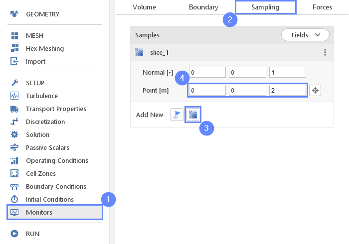
19. Monitors - Sampling (I)
During the calculation, we can observe intermediate results on a section plane. To add sampling data on a plane we need to define plane properties and also select fields that will be sampled. We will monitor the pressure and velocity at a height of 2 metres from the ground. Note that runtime post-processing can only be defined before starting calculations and can not be changed later on.
- Go to Monitors panel
- Switch to Sampling tab
- Select Create Slice
- Set slice plane location
Point \({\sf [m]}\)002
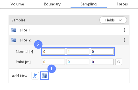
20. Monitors - Sampling (II)
Now, create a vertical slice.
- Select Create Slice
- Select slice_2
- Set slice normal vector
Normal \({\sf [-]}\)010
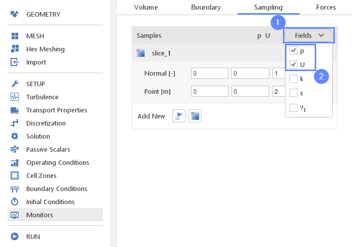
21. Monitors - Sampling (II)
Now, specify which results should be sampled on the section planes.
- Expand Fields list
- Select pressure p and velocity U
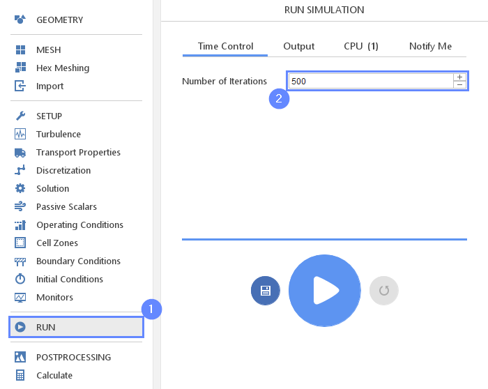
22. Run - Time Control
Finally, we can start our computation.
- Go to RUN panel
- Set the maximum Number of Iteration to 500
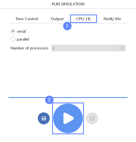
23. Run - CPU
To speed up the calculation process, take advantage of parallel computing and increase the number of CPUs based on your PC’s capability. The free version allows you to use only one processor (serial mode). To get the full version, you can use the contact form to Request 30-day Trial
Estimated computation time for serial mode: 5 minutes
- Switch to CPU tab
- Click Run Simulation button
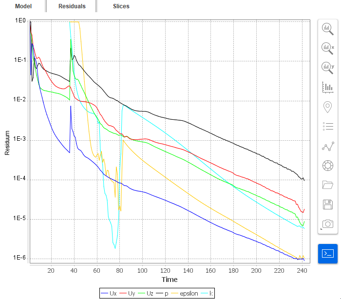
24. Residuals
When the calculation is finished, we should see a similar residual plot.
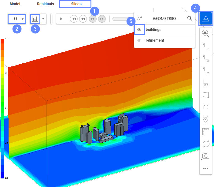
25. Slice - Velocity Field
Slices tab appears next to the Residuals tab. Under this tab, we can preview results on the defined section plane.
- Change tab to Slices
- Select the velocity U
- Click Adjust range to data
- Click Graphics Object List icon
- Navigate to GEOMETRIES
- Show the buildings
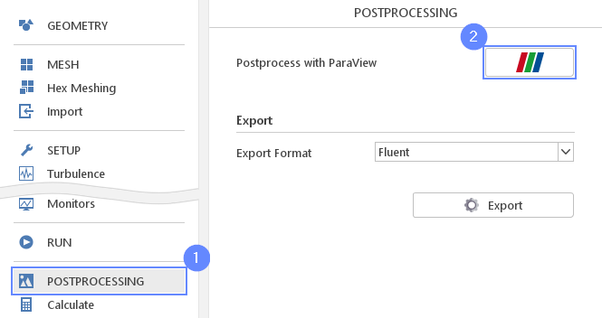
26. Postprocessing - ParaView
After computations are finished, we can do complex visualization of our results with ParaView.
- Go to Postprocessing panel
- Start ParaView
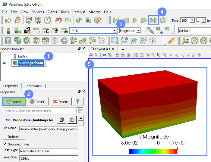
27. ParaView - Load Results
Load the results into the program.
- Make sure you have your case selected buildings.foam
- Click Apply to load results
- Select contour coloring variable to U
- Click Last Frame to load the final result set
- After loading results they will be shown in the 3D graphic window
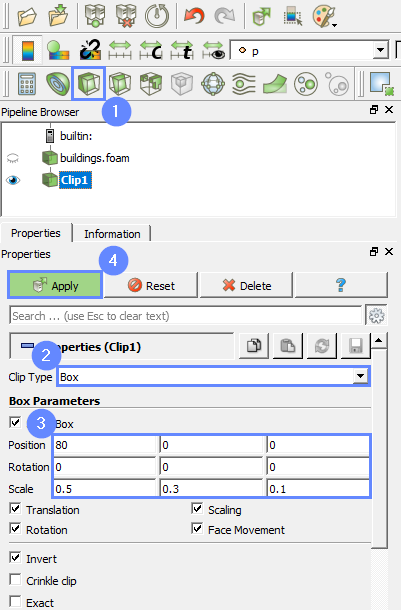
28. ParaView - Clip
To limit the investigation area we will Clip the domain by the box.
- Select Clip option
- Change the Clip Type to Box
- Enter box parameters accordingly
Position-70-900
Rotation000
Lenght40018040 - Click Apply
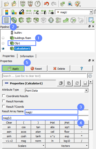
29. ParaView - Velocity Field
Now we will create velocity magnitude parameter. It will be helpful in scaling and coloring the velocity vector field.
- Make sure you have Clip1 field selected
- Select Calculator
- Type the magU as Result Array Name
- Type the formula mag(U)
- Click Apply
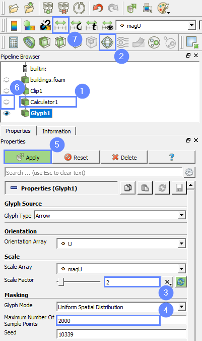
30. ParaView - Velocity Field Settings
To visualize the flow around the building we will create vector field.
- Make sure you have Calculator1 field selected
- Select Glyph option
- Set the scale factor to 2
- Change the Maximum Number Of Sample Points to 2000
- Click Apply
- Hide the Calculator1 field
- Click Rescale to Data Range
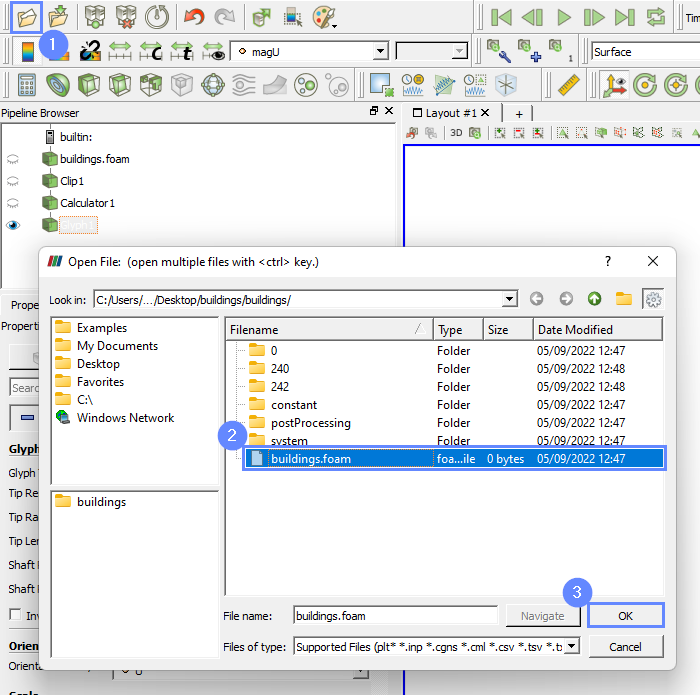
31. ParaView - Import Geometry (I)
To display results with the original geometry, we can import the case once again and select only suitable boundaries. Now, we will import the buildings and the ground boundaries.
- Click Open
- Select the buildings.foam file from the case directory …/buildings/buildings/buildings.foam
- Click OK button
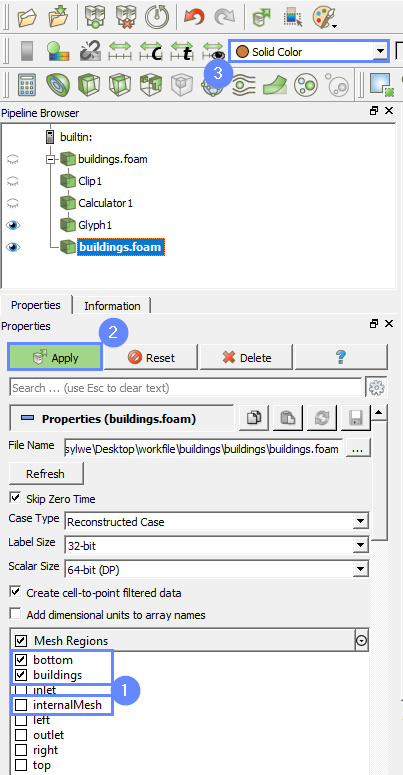
32. ParaView - Import Geometry (II)
- Check bottom and buildings instead internalMesh boundary
- Click Apply button to show the geometry
- Set the coloring as Solid Color
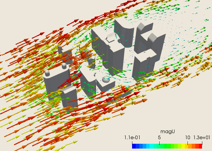
33. ParaView - Display Velocity Field
Now we can see the velocity vector field around the buildings.
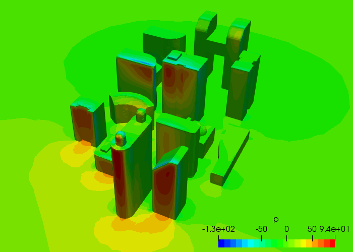
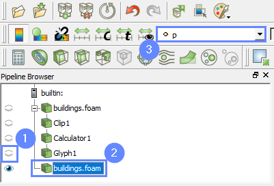
34. ParaView - Pressure on Buildings (I)
To display pressure on the buildings we need to hide vector field and change the coloring to the pressure.
- Hide the Glyph1
- Select buildings.foam field (with the buildings and ground boundaries)
- Change the coloring set to pressure p
35. ParaView - Pressure on Buildings (II)
Pressure field is displayed on the selected boundaries.