3. Create Case
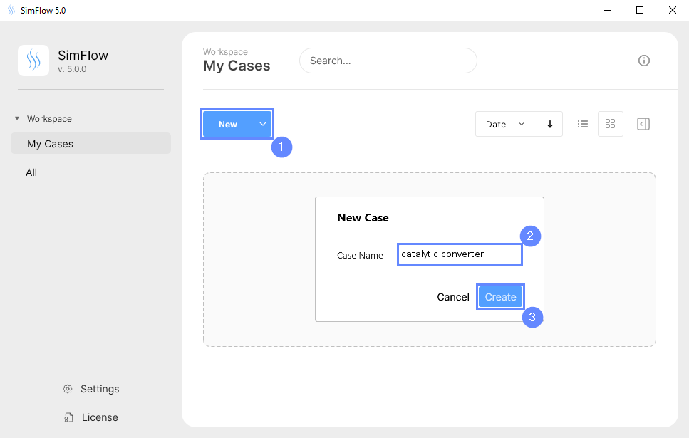
Open SimFlow and create a new case named catalytic converter
- Click New
- Provide name catalytic converter
- Click Create to open a new case
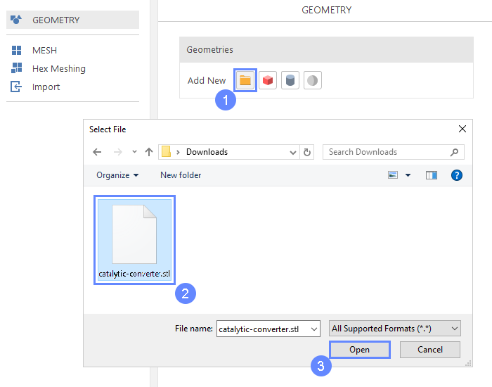
4. Import Geometry
Firstly we need to Download GeometryCatalytic-converter
- Click Import Geometry
- Select geometry file catalytic-converter.stl
- Click Open to import geometry
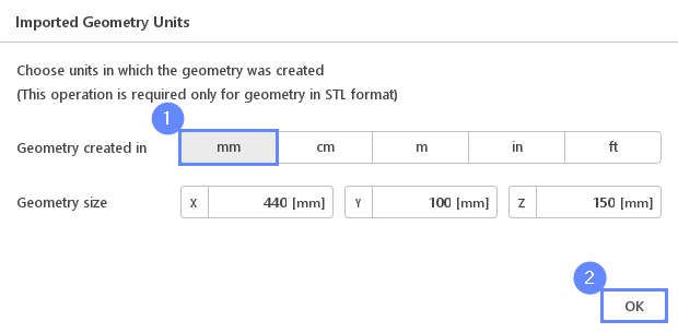
5. Imported Geometry Units
Since the imported geometry is in STL format, which does not store unit information, we need to confirm the unit in which the model was created. In the selection of unit, we can use the Geometry size label, which displays the overall size of the model in each direction. In our case, the model was created in millimeters.
- Select mm unit
- Press OK button
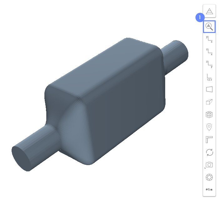
6. Geometry - Catalytic Converter
After importing geometry, it will appear in the 3D window.
- Click Fit View to zoom in on the geometry
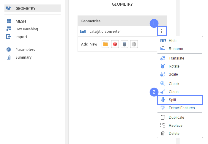
7. Split Geometry - Catalytic Converter (I)
The imported geometry is made up of a single surface. We need to split it into multiple faces for further processing.
- Expand the Options list for catalytic_converter
- Select Split
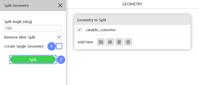
8. Split Geometry - Catalytic Converter (II)
In order to split original geometry into separate objects, we will disable Create Single Geometry options:
- Uncheck Create Single Geometry
- Click Split
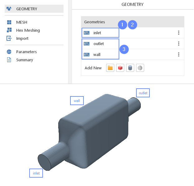
9. Rename Geometries
To make the mesh boundaries easier to recognize, we will rename each geometry face as follows:
- Double-click each geometry name in the list and rename it accordingly:
catalytic_converter_patch00 \(\rightarrow\) inlet
catalytic_converter_patch01 \(\rightarrow\) outlet
catalytic_converter_patch02 \(\rightarrow\) wall
As you select each face, it will be highlighted in the 3D graphics window. Ensure that the renamed faces match the reference shown in the image below.
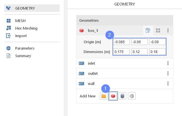
10. Create Geometry - Cell Zone
In this tutorial, we would like to model a porous zone inside the catalytic converter. To do so we need to define the region where the porous resistance will be applied. For this purpose we will create new box geometry:
- Click on Create Box
- Set the origin and box dimensions accordingly
Origin \({\sf [m]}\)-0.085-0.06-0.09
Dimensions \({\sf [m]}\)0.1750.120.18
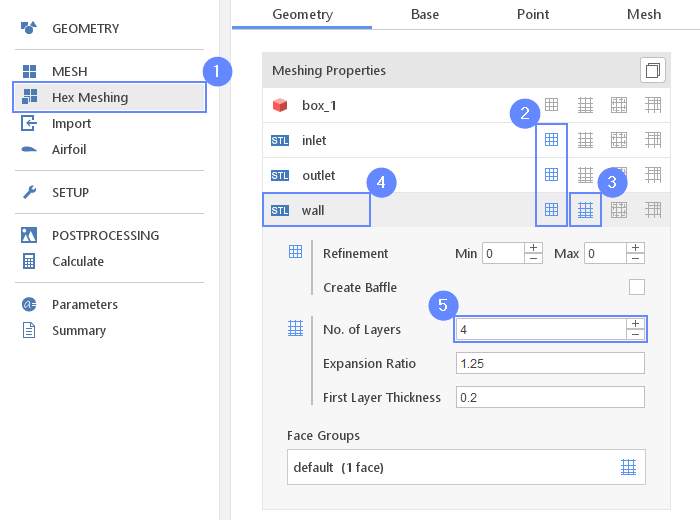
11. Meshing Properties - Catalytic Converter
In order to create the mesh, we need to specify geometries options used during the meshing process.
- Go to Hex Meshing panel
- Enable Mesh Geometry on the inlet outlet wall
- Enable Create Boundary Layer Mesh on wall geometry
- Click on the wall in the list to expand options
- Set No. Of Layers to 4
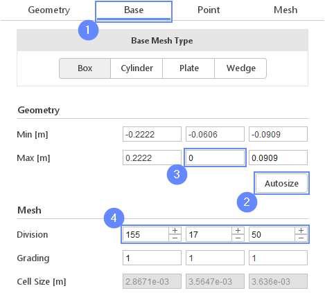
12. Base Mesh - Domain
Now we will define the base mesh. The box geometry determines the background mesh domain. The model is symmetrical on the XZ plane, so we do not need to mesh the whole geometry. Using the box dimensions, we will choose only half of the domain.
- Go to Base tab
- Click on Autosize
- Change Max [m] Y to 0
- Define the number of divisions
Division1551750
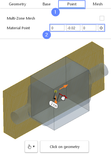
13. Material Point
Material Point tells the meshing algorithm on which side of the geometry the mesh is to be retained. Since we are considering flow inside the catalytic converter we need to place the material point inside the geometry.
- Go to Point tab
- Specify location inside the catalytic converter geometry
Material Point0-0.020
You can specify the point location from the 3D view. Hold the CTRL key and drag the arrows to the destination.
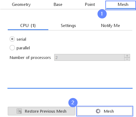
14. Start Meshing
Everything is now set up for meshing
- Go to Mesh tab
- Start the meshing process with Mesh button
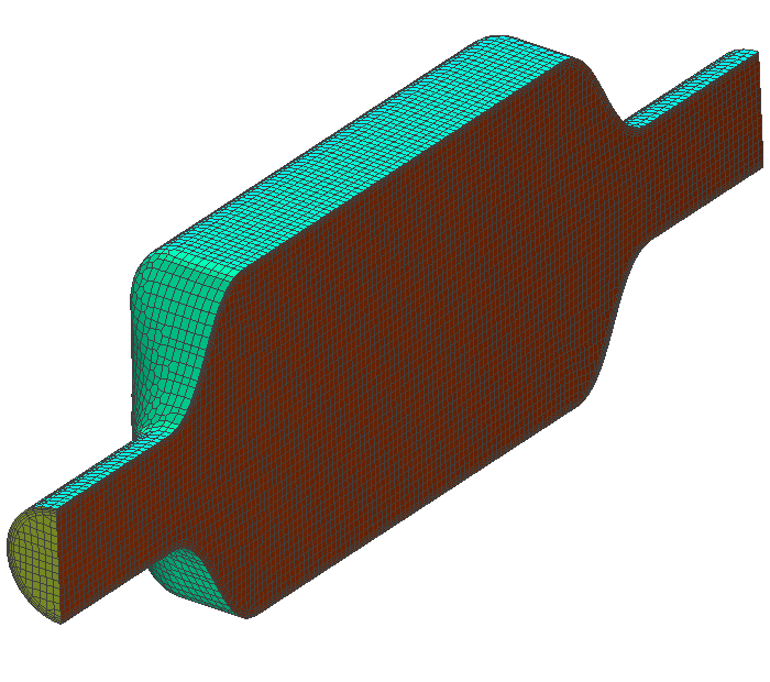
15. Mesh
After the meshing process is finished the mesh will appear in the graphics window.
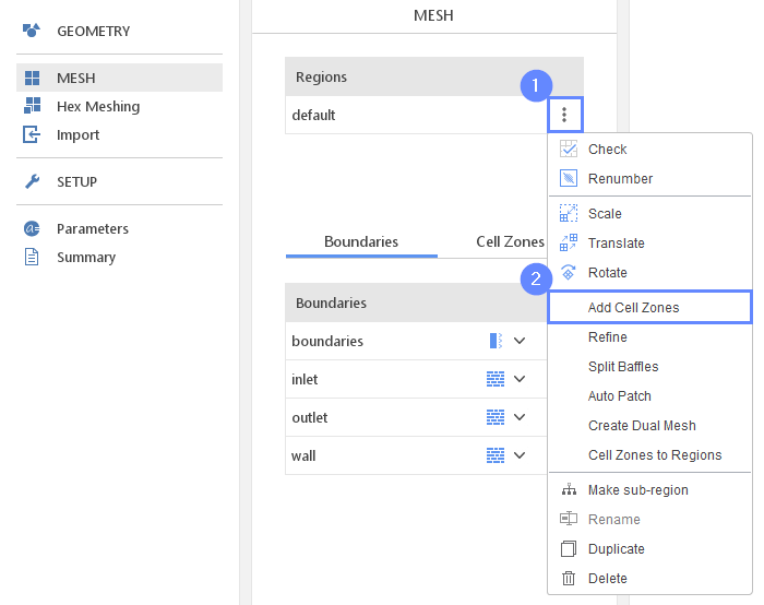
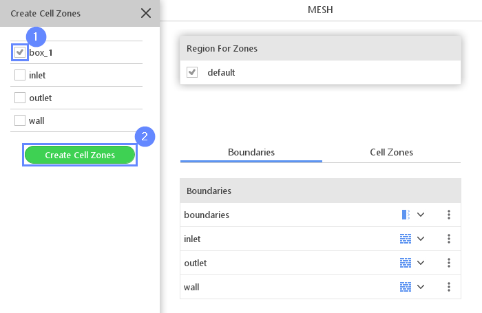
16. Create Cell Zone (I)
Now we will define the cell zone using box_1 geometry.
- Expand the Options list next to default region
- Select Add Cell Zones
17. Create Cell Zone (II)
- Check the box_1
- Click on Create Cell Zones
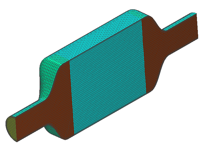
18. Display Cell Zone
The cell zone appears inside the catalytic converter. It is colored on light blue.
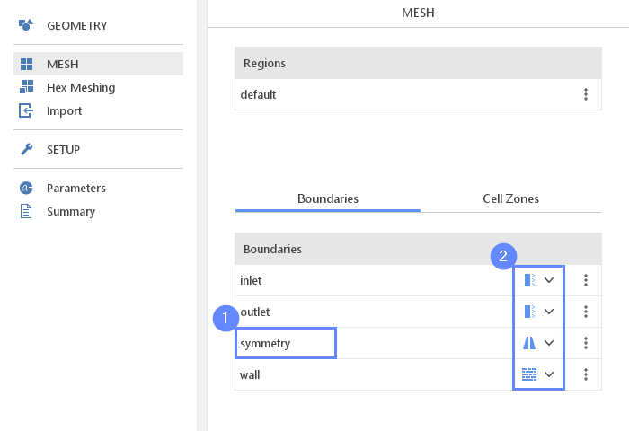
19. Boundaries
- Change boundary name
boundaries \(\rightarrow\) symmetry - Define boundary types accordingly
inlet Patch
outlet Patch
symmetry Symmetry
wall Wall
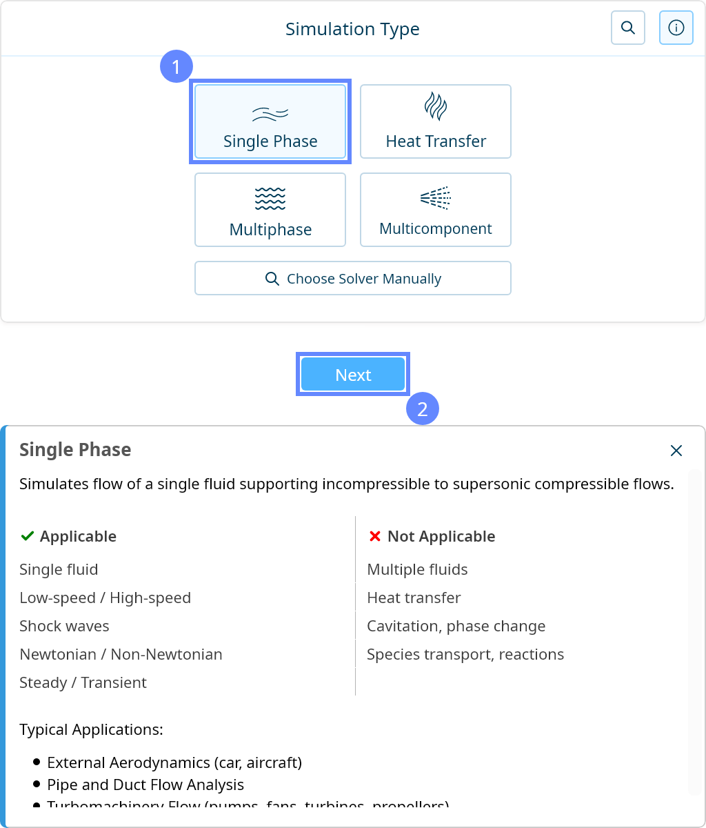
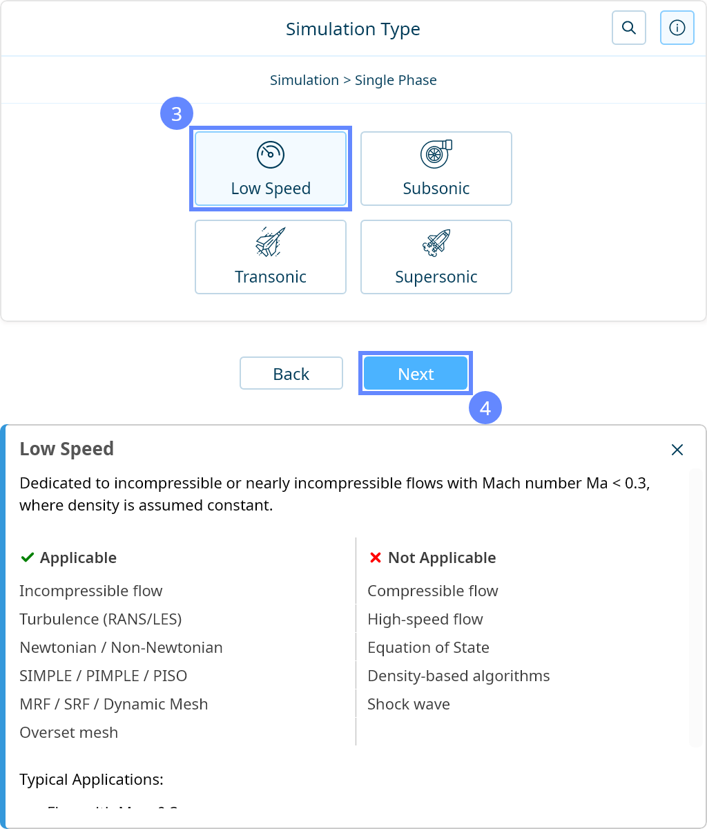
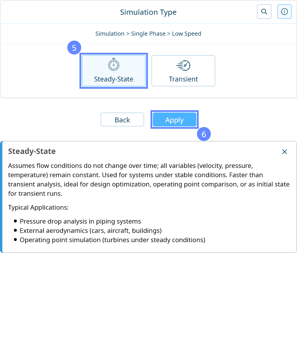
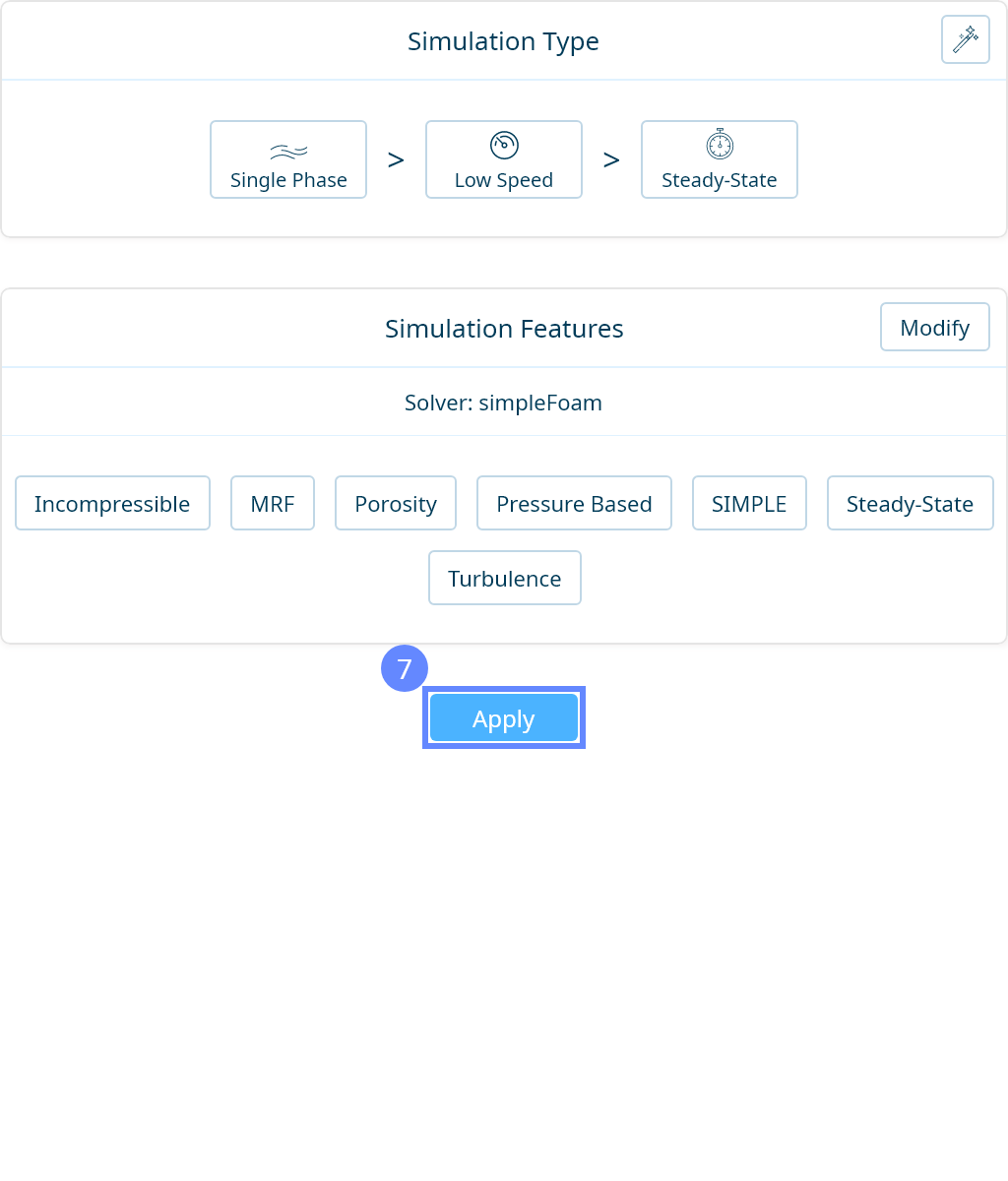
20. Simulation Type
We want to analyze internal, incompressible turbulent flow. For this purpose, we will use a single-phase, steady-state simulation of incompressible turbulent flow.

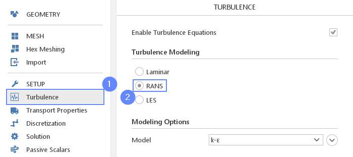
21. Turbulence
For turbulence modeling, we will use the standard \(k-\varepsilon\) model.
- Go to Turbulence panel
- Select RANS for Turbulence Modeling
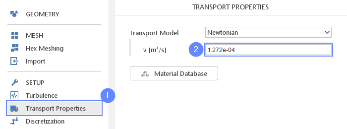
22. Transport Properties
We will change the kinematic viscosity to the value of the exhaust gas.
- Go to Transport Properties panel
- Set the kinematic viscosity
\(\nu\) \({\sf [\frac{m^2}{s}]}\)1.272e-04
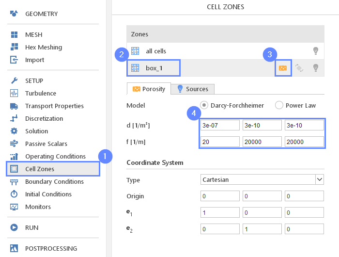
23. Cell Zones - Porosity
In order to include porosity to our simulation we have to define porosity for the box_1 cell zone.
- Go to Cell Cones panel
- Select the box_1 zone
- Check Porous Zone
- Use default Darcy-Forchheimer model and set its parameters accordingly
d \({\sf [\frac{1}{m^2}]}\)3e-073e-103e-10
f \({\sf [\frac{1}{m}]}\)202000020000
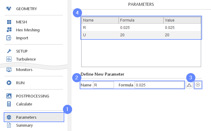
24. Parameters - R, U
SimFlow allows users to create named parameters that can be used instead of numbers. This allows to easily change a single property without the need to edit all inputs where a given property is used. In this tutorial, we will define two global parameters that we will use during further setup.
- Go to Parameters panel
- Definethe new parameter
Name R Formula 0.025 - Click Create Parameter
- Repeat these steps for the second parameter
Name U Formula 20
The newly created parameters will be shown in the parameters list.
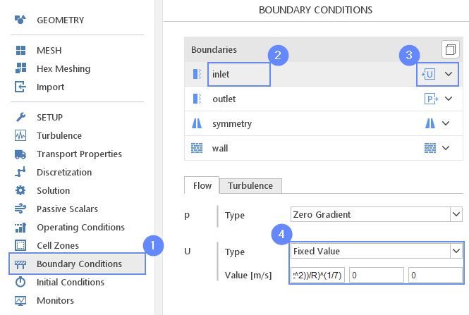
25. Boundary Conditions - Inlet (Flow)
We will set inlet velocity as a parabolic profile. The profile we will define by the formula using U and R parameters. Velocity magnitude near the wall will be equal to zero and the highest value of U will be in the center of the pipe.
- Go to Boundary Conditions panel
- Select the inlet boundary
- Set the Velocity Inlet character
- Change the velocity type and value accordingly
U Type Fixed Value
U Value \({\sf [\frac{m}{s}]}\)U*( (R-sqrt(y^2 +z^2 ))/R)^(1/7)00
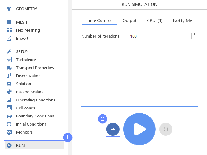
26. Save Case
To visualize and check velocity distribution we will open ParaView. Firstly we will save the case.
- Go to RUN panel
- Press Save Case button
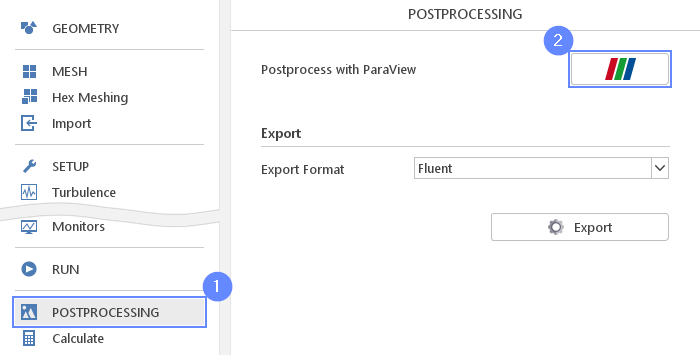
27. Check Velocity Profile - ParaView (I)
Run the ParaView from the Postprocessing panel.
- Go to POSTPROCESSING panel
- Click on Run ParaView
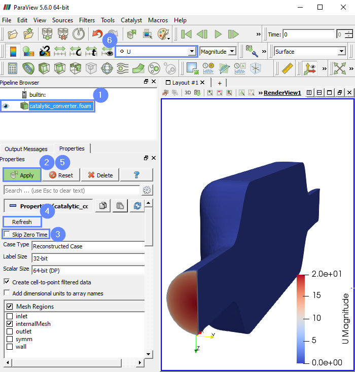
28. Check Velocity Profile - ParaView (II)
We will display a velocity magnitude map on the inlet.
- Make sure that catalytic_converter is selected
- Press Apply
- Uncheck Skip Zero Time
- Press Refresh
- Press Apply
- Select velocity U from the list
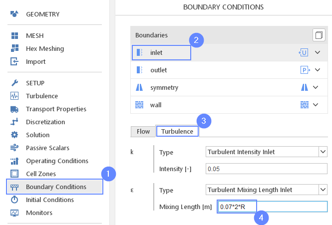
29. Boundary Conditions - Inlet (Turbulence)
Back in SimFlow, we will also update the turbulent mixing length for the ε-equation at the inlet.
- Go to Boundary Conditions panel
- Select inlet boundary
- Switch to Turbulence tab
- Set the value of Mixing Length to 7% of inlet diameter
\(\varepsilon\) Mixing Length \({\sf [m]}\)0.07*2*R
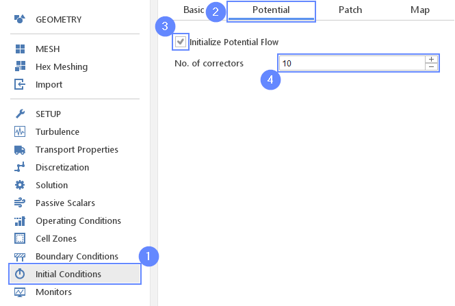
30. Initial Conditions - Potential
In order to give a better initial guess for velocity and pressure fields, we will use the "Potential" initialization feature. This utility solves pseudo potential flow prior to actual calculations.
- Go to Initial Conditions panel
- Switch to Potential tab
- Check the Initialize Potential Flow
- Set No. of correctors to 10
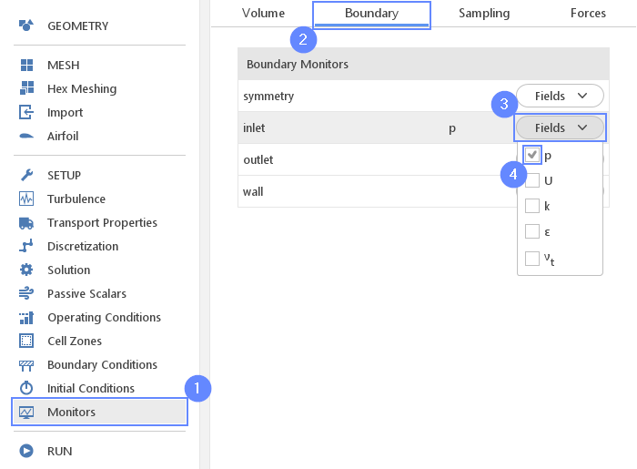
31. Monitors - Boundary
We would like to monitor how results change during computation. We will enable plotting the average pressure at the inlet during the calculation:
- Go to Monitors panel
- Switch to Boundary tab
- Expand Fields list next to inlet boundary
- Check the pressure p
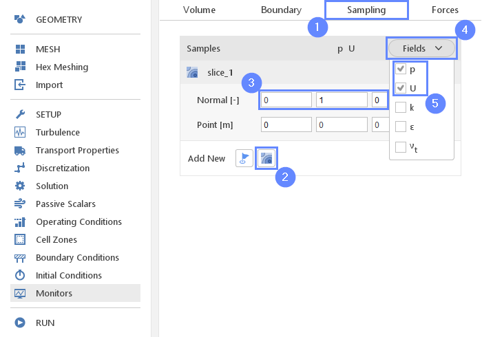
32. Monitors - Sampling
We will also display intermediate results on a section plane.
- Go to Sampling tab
- Add new Slice
- Set the normal vector
Normal \({\sf [-]}\)010 - Expand Fields menu
- Choose the pressure p and the velocity U to be sampled on the section plane
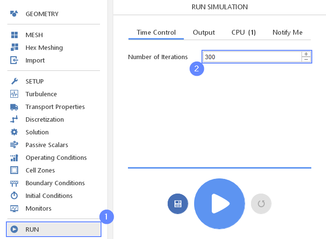
33. Run - Time Control
- Go to RUN panel
- Set the maximal Numbers of Iterations to 300
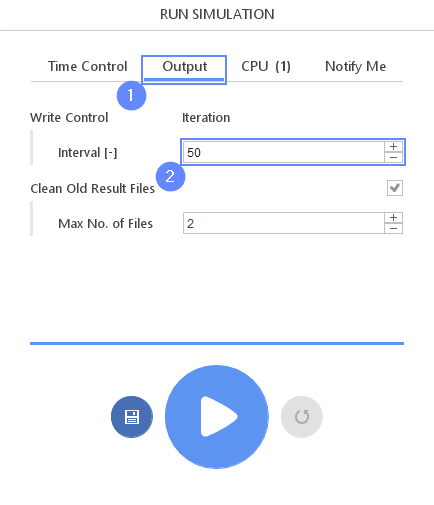
34. Run - Output
In this tutorial, we will run a steady-state simulation, where only the final solution is of interest. In this tab, you can specify how frequently intermediate results are displayed during the calculation. Set the preview interval to 50 iterations.
- Switch to Output tab
- Set the Interval [-] to 50
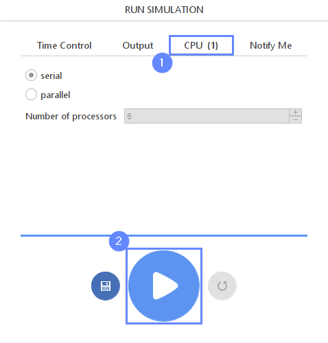
35. Run - CPU
To speed up the calculation process, take advantage of parallel computing and increase the number of CPUs based on your PC’s capability. The free version allows you to use only one processor (serial mode). To get the full version, you can use the contact form to Request 30-day Trial
Estimated computation time for serial mode: 8 minutes
- Switch to CPU tab
- Click Run Simulation button
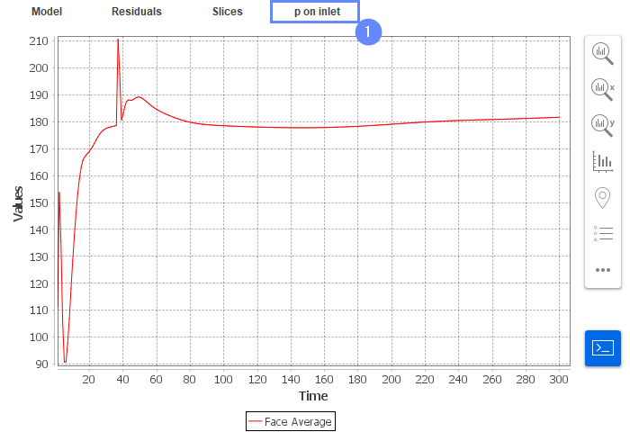
36. Control Inlet Pressure
Go to the p on inlet tab to observe convergence process.
- Switch to p on inlet tab
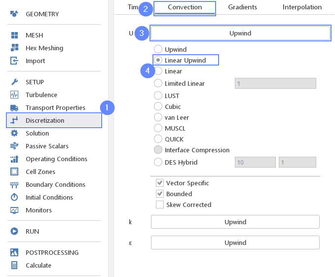
37. Discretization
After preliminary calculation, we will continue with a more accurate algorithm. Change velocity discretization to the Linear Upwind scheme to minimize numerical diffusion affecting results of the simulation.
- Go to Discretization panel
- Switch to Convection tab
- Click on Upwind to extend the list
- Select Linear Upwind
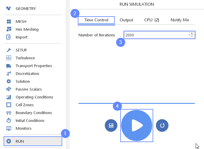
38. Run - Continue Simulation
- Go to RUN panel
- Set the maximal Numbers of Iterations to 2000
- Click Continue Simulation button
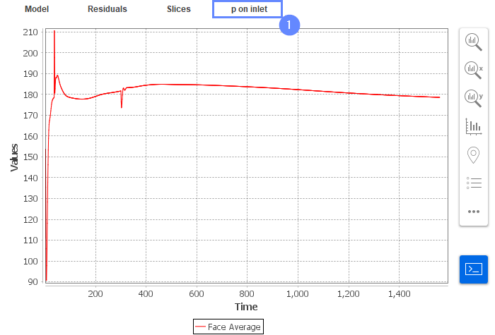
39. Control Inlet Pressure - New Scheme
Go back to the p on inlet tab and observe convergence process.
- Switch to p on inlet tab
- Control the convergence of the pressure on the inlet
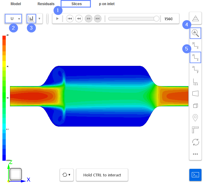
40. Slice - View Velocity Field
Slices tab appears next to the Residuals tab. Under this tab, we can preview results on the defined section plane.
- Change tab to Slices
- Select the velocity U
- Click Adjust range to data
- Click Fit View
- Set the XZ orientation View XZ
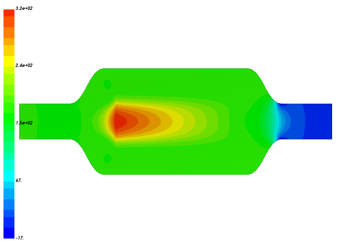
41. Slice - Final Results
At the end, we will look at the pressure distribution. The Darcy porous model assumes resistance and hence pressure gradient to be proportional to the velocity in the porous zone. We can observe the effect of increased resistance from the porous zone. The pressure builds up in front of the porous zone and then linearly decreases along the flow direction due to resistance.