3. Create Case
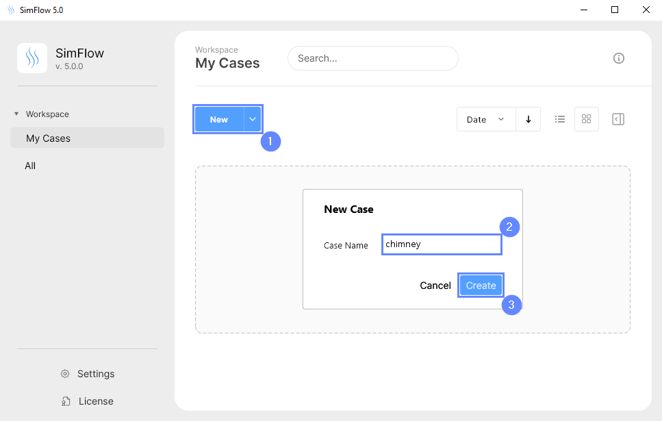
Open SimFlow and create a new case named chimney
- Click New
- Provide name chimney
- Click Create to open a new case
4. Create Geometry - Chimney
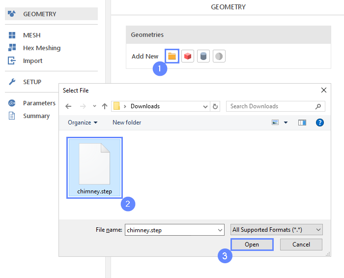
Firstly, we need to Download GeometryChimney
The geometry will be imported in the same units as it was exported to the STEP format.
- Click Import Geometry
- Select geometry file chimney.step
- Click Open
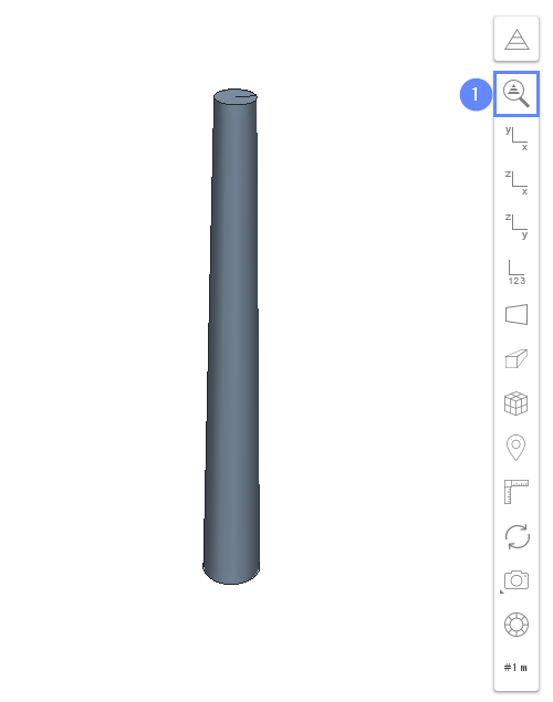
5. Geometry - Chimney
The resulting geometry will be displayed in the graphics window.
- Click Fit View to zoom in the geometry
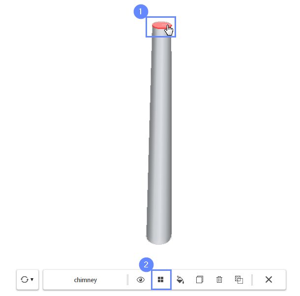
6. Creating Face Group - Inlet 1
In this simulation, we are dealing with an external flow problem. The imported chimney geometry serves as an airflow obstacle and introduces a second phase into the domain. To define where the boundaries of the inlet mesh should be created, we will use the Face Groups.
- Select the inlet face by holding CTRL key and clicking on the geometry face in a 3D view. The selection should be marked in red
- Click on the Face Group button in the graphics context toolbar
- Press Esc key to clear the selection
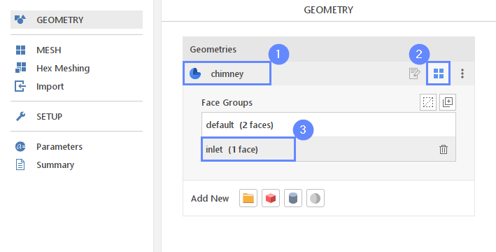
7. Rename Face Group
In the Geometry Panel, find the new Face Group under the chimney geometry. The first group, named default, contains all non-selected surfaces, which will become the chimney walls.
The new group represents the contaminant inlet to the domain. Rename this group to inlet.
- Select chimney geometry
- Expand Geometry Faces
- Change face group name (double-click on a group name to start editing)
group_1 \(\rightarrow\) inlet
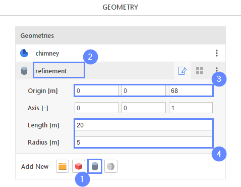
8. Geometry - Refinements (I)
To achieve a denser mesh at the chimney outlet and in the region of contaminant dispersion, we will create two geometries to specify the areas for mesh refinement.
- Select Create Cylinder
- Rename it to refinement
(double click on the geometry name to start rename) - Set the cylinder origin:
Origin \({\sf [m]}\)0068 - Set the cylinder dimensions:
Length \({\sf [m]}\)20
Radius \({\sf [m]}\)5
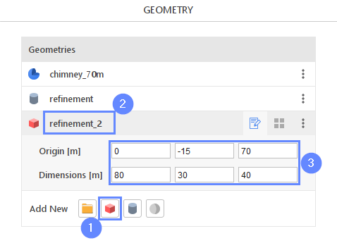
9. Geometry - Refinements (II)
- Select Create Box
- Rename it to refinement_2
- Set the box origin and dimensions:
Origin \({\sf [m]}\)0-1570
Dimensions \({\sf [m]}\)803040
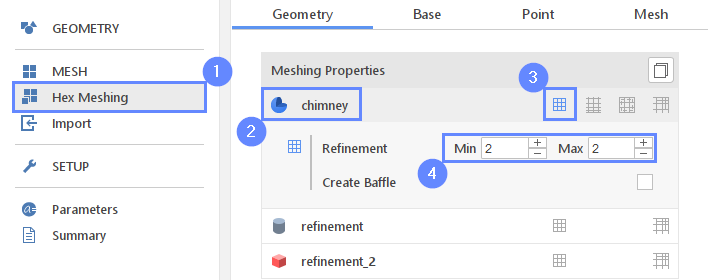
10. Meshing Parameters - Chimney
To create the mesh, we need to specify the meshing options for the given geometry. For the chimney, we will refine the mesh near its faces.
- Go to Hex Meshing panel
- Select the chimney component
- Enable Mesh Geometry
- Set Refinement to Min 2 Max 2
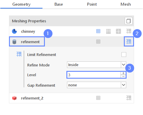
11. Meshing Parameters - Refinement I
For the refinement geometry, we will set the mesh refinement inside the volume.
- Select the refinement component
- Enable Refine Geometry
- Set refinement Level to 3
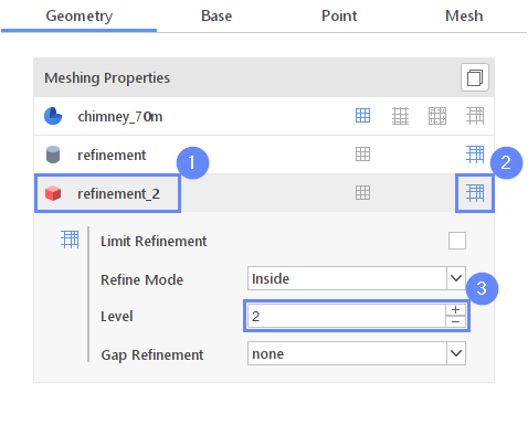
12. Meshing Parameters - Refinement II
- Select the refinement_2 component
- Enable Refine Geometry
- Set refinement Level to 2
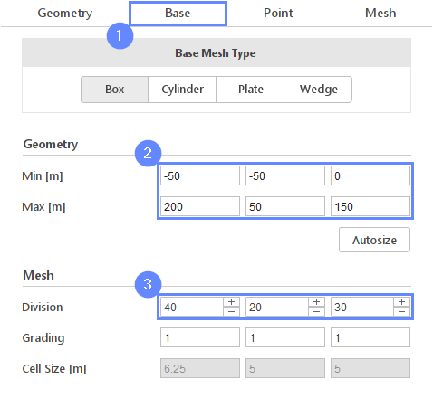
13. Base Mesh - Domain
As we are considering an external flow, the area under consideration is limited by the size of the base mesh domain. For this purpose, we will use a Box base mesh type.
- Go to Base tab
- Set the base mesh size:
Min \({\sf [m]}\)-50-500
Min \({\sf [m]}\)20050150 - Define the number of divisions
Division402030
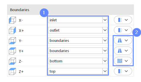
14. Base Mesh Boundaries
Now, we need to assign individual names to each side of the base mesh to define different conditions on each side. We will use symmetry as a boundary type for simplified slip conditions on the side and top boundaries.
- Define boundary names accordingly
X- inlet
X+ outlet
Y- boundaries
Y+ boundaries
Z- bottom
Z+ top - Define boundary types accordingly
Y- Symmetry
Y+ Symmetry
Z- Wall
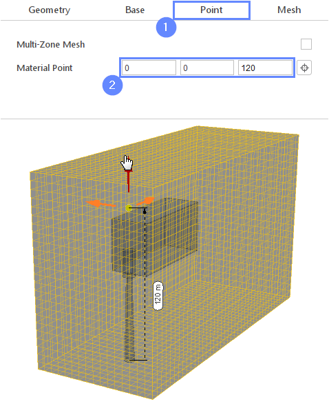
15. Material Point
The material point indicates on which side of the geometry the mesh is to be retained. We are simulating flow around the chimney, so our material point needs to be located inside the base mesh but outside the chimney.
- Go to Point tab
- Specify location inside base mesh but outside chimney geometry
Material Point00120
You can specify the point location from the 3D view. Hold the CTRL key and drag the arrows to the destination.
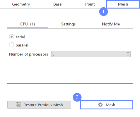
16. Start Meshing
In this step, we will initiate the meshing process.
In the meshing panel, you can indicate how many CPUs you would like to use for this process. Note that if you are using the free version of SimFlow, you may only use serial meshing and cannot create meshes larger than 200,000 nodes.
If you would like to test full version Request 30-day Trial
- Switch to Mesh tab
- Start the meshing process with Mesh button
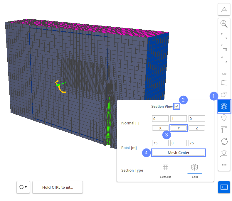
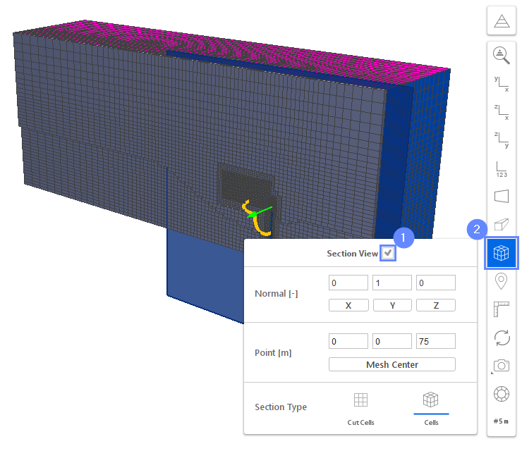
17. Mesh
After the meshing process is finished, the mesh should appear on the screen. To control the mesh quality inside the domain, we can enable cross-section view.
- Select Section View
- Mark Section View
- Set section plane normal along Y axis
- Click Mesh Center to locate the section plane in the center of the model
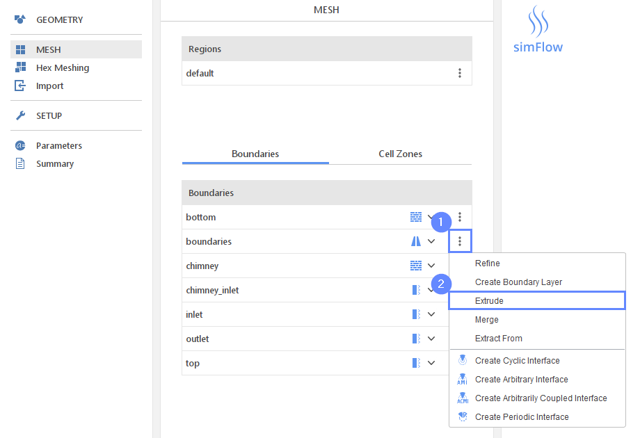
18. Domain Extrusion - Sides (I)
With SimFlow, you can modify the existing mesh domain by extending the volume through boundary extrusion. This allows the size of successive mesh cells to be graded. For this tutorial, we will extend the domain on each side.
At the beginning, extrude the sides of the boundaries.
- Expand the Options list for the boundaries
- Select Extrude option
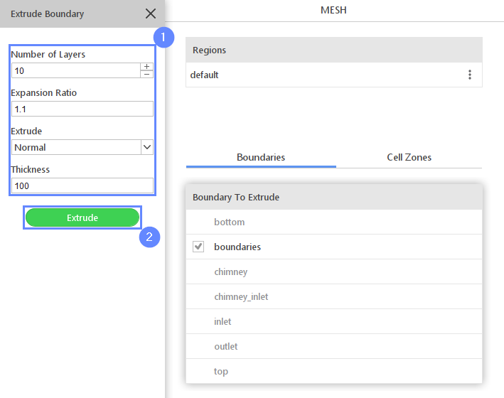
19. Domain Extrusion - Sides (II)
Selected boundaries will be extended by 100 meters in the normal direction. The additional mesh will be split into 10 rows of cells in the extrusion direction with a grading of 1.1.
- Set the following parameters accordingly:
Number of Layers10
Expansion Ratio1.1
ExtrudeNormal
Thickness100 - Click Extrude
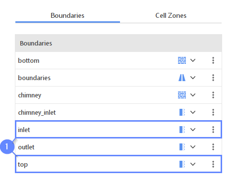
20. Domain Extrusion - Inlet and Top
Next, repeat the extrusion process for the Inlet and Top boundaries using the same parameters as before.
- Select the Inlet boundary and Extrude it using the previously defined parameters
- Repeat the Extrude operation for the Top boundary
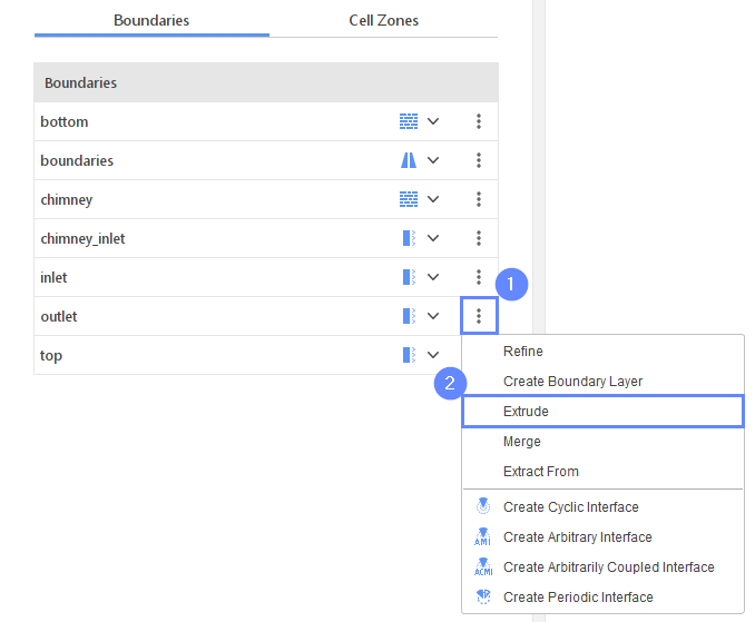
21. Domain Extrusion - Outlet (I)
For extrusion of the Outlet boundary, we will use a different set of parameters.
- Expand the Options list for the outlet
- Select Extrude option
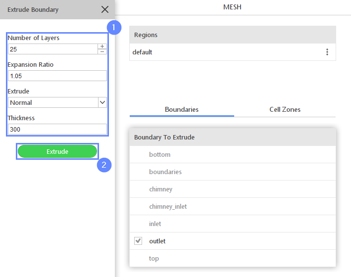
22. Domain Extrusion - Outlet (II)
The outlet boundary will be extended by 300 meters, spliting an extra volume on 25 rows of cells with an expansion ratio of 1.05.
- Set the following parameters accordingly:
Number of Layers25
Expansion Ratio1.05
ExtrudeNormal
Thickness300 - Click Extrude
23. Mesh Investigation
Using the expansion ratio allows you to significantly enlarge the domain without significantly increasing the number of cells.
Now, we can disable the section view.c
- Uncheck the Section View option
- Close the toolbox by clicking the Section View icon
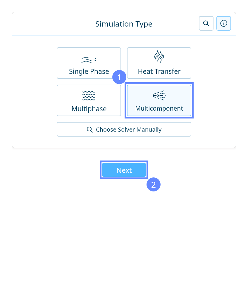
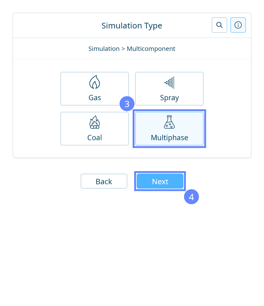
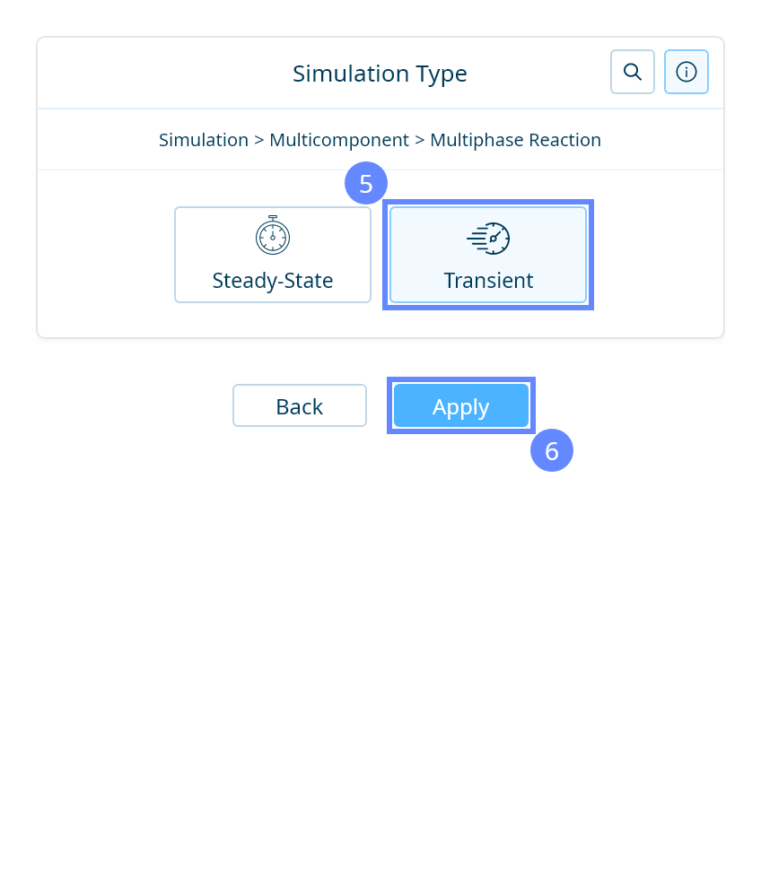
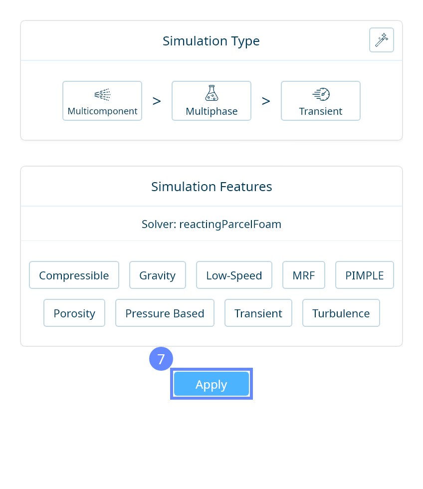
24. Simulation Type
We want to analyze a compressible, turbulent flow involving multiple gases and solid particles. For this purpose, we will use a transient simulation with species transport and particle tracking.

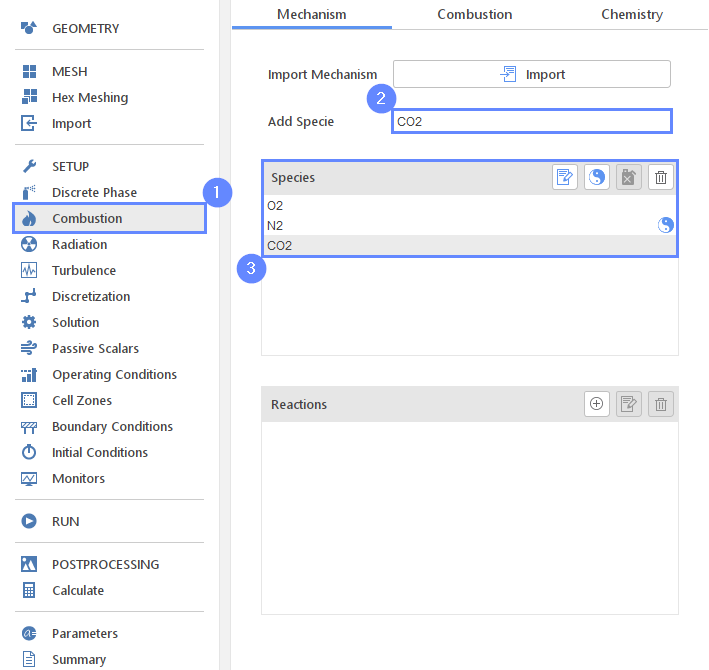
25. Combustion - Mechanism
We are going to model a dispersion of carbon dioxide in the atmosphere. Therefore, we will need three species to model this: nitrogen, oxygen and carbon dioxide.
- Go to Combustion panel
- Add the missing species by typing its chemical formula and selecting it from the list:
Add SpeciesCO2 - Check if all necessary species are listed
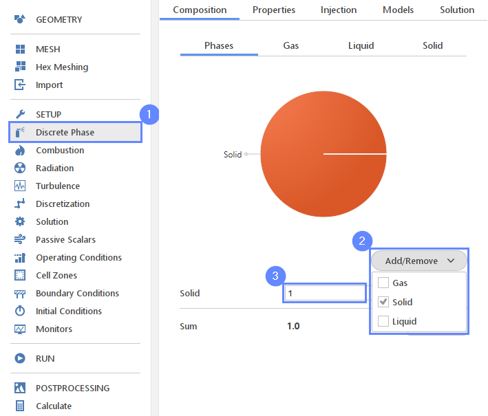
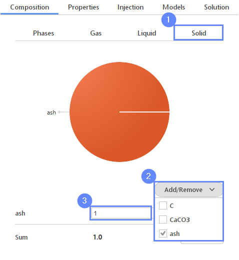
26. Discrete Phase - Composition
We will consider a second type of pollutants, which involves solid particles such as ash emitted from the chimney. To initiate this process, we will define the solid phase of the Lagrangian particles in the Discrete Phase panel.
- Go to Discrete Phase panel
- Extend Add/Remove list
- Check Solid phase and uncheck the Liquid
27. Discrete Phase - Material
Now, select the ash as a material of particles.
- Switch tab to Solid
- Extend Add/Remove list, check ash phase and uncheck the others
- Set ash fraction to 1
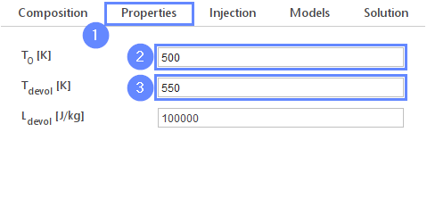
28. Discrete Phase - Properties
Next, define the initial temperature of the particles.
- Switch tab to Properties
- Define ash temperature
\(T_0\) \({\sf [K]}\)500 - Define devolatilization temperature
\(T_{devol}\) \({\sf [K]}\)550
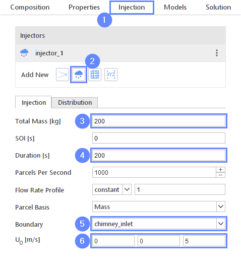
29. Discrete Phase - Injection
We will now define the injection of the discrete phase through the chimney inlet boundary. We assume a constant flow rate of 100 kg of ash over 100 s, with the particle velocity equal to the gas velocity escaping from the chimney.
- Go to Injection tab
- Create Boundary Injector
- Set the total mass of the particles
Total Mass \({\sf [kg]}\)200 - Set the duration of injecting particles
Duration \({\sf [s]}\)200 - Select the boundary to be injected from
Boundarychimney_inlet - Define the inlet velocity of the particles
\(U_0\) \({\sf [m/s]}\)005
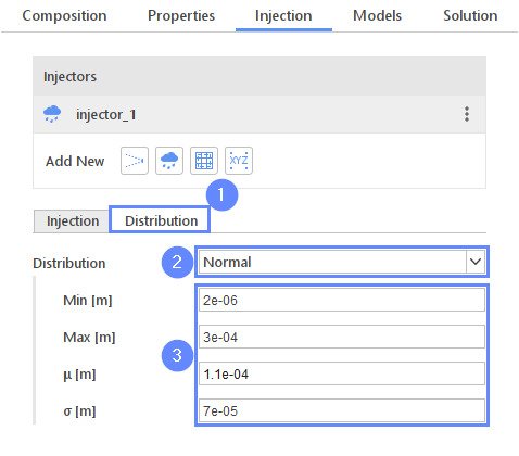
30. Discrete Phase - Distribution
In this step, define the particle size using a normal distribution.
- Go to Distribution tab
- Set Distribution to Normal
- Set distribution parameters accordingly
Max \({\sf [m]}\)2e-06
Max \({\sf [m]}\)3e-04
\(\mu\) \({\sf [m]}\)1.1e-04
\(\sigma\) \({\sf [m]}\)7e-05
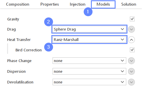
31. Discrete Phase - Models
We need to define which models will be used in this simulation. We select the Sphere Drag model to account for the drag force acting on the droplets. The Ranz-Marshall heat transfer model is used to consider heat transfer between the particles and surrounding gas.
- Switch to Models tab
- Set the drag model as Sphare Drag
- Set the heat transfer model as Ranz-Marshall
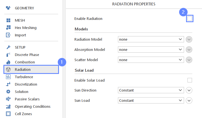
32. Radiation
We will disable radiation for our simulation.
- Go to Radiation panel
- Uncheck Enable Radiation option
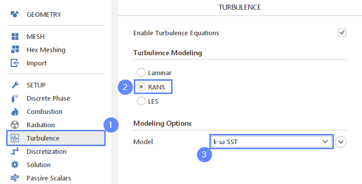
33. Turbulence
We are going to use the standard \(k{-}\omega \; SST\) model to resolve turbulence.
- Go to Turbulence panel
- Select RANS modeling
- Select \(k{-}\omega \; SST\) model
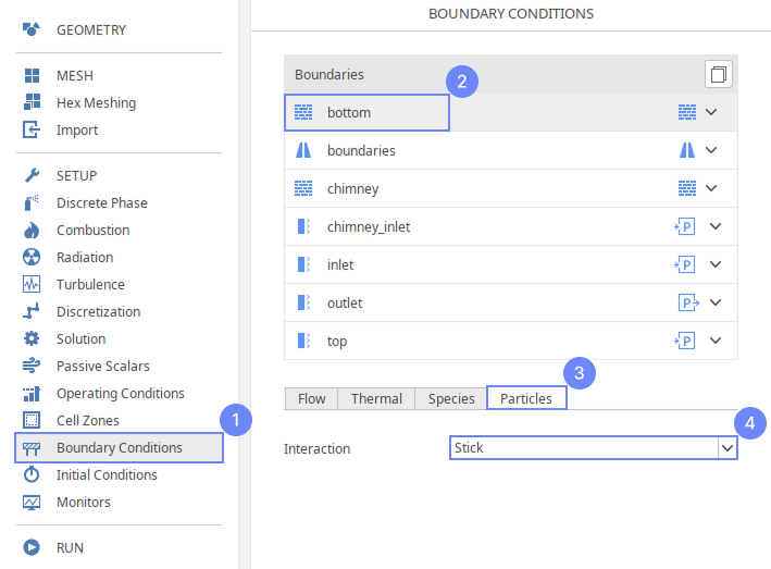
34. Boundary Conditions - Bottom
Now, we will define the boundary conditions. First, we will specify the particle behavior at the bottom boundary as Sticky.
- Go to Boundary Conditions panel
- Select bottom boundary
- Switch tab to Particles
- Set Interaction to Stick
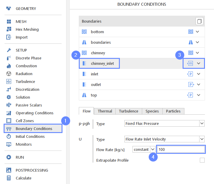
35. Boundary Conditions - Chimney Inlet
For the chimney_inlet, we will set a constant CO2 flow rate.
- Select chimney_inlet boundary
- Set the Mass Flow Inlet character
- Switch tab to Flow
- Set the flow rate
U Flow Rate \({\sf [kg/s]}\)100
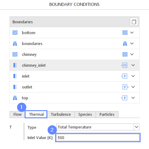
36. Boundary Conditions - Chimney Inlet - Thermal
- Go to Thermal boundary conditions tab
- Set the temperature: T Inlet Value \({\sf [K]}\)500
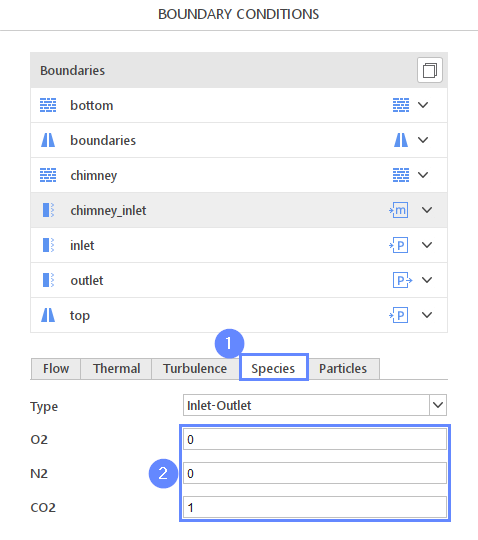
37. Boundary Conditions - Chimney Inlet - Species
Define the phase fractions of the escaping gas. The sum of all shares must be equal to 1.
- Switch tab to Species
- Set the inlet phase:
O20
N20
CO21
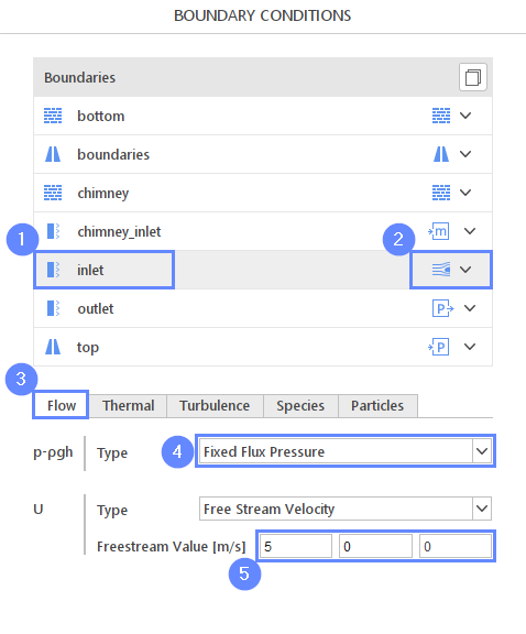
38. Boundary Conditions - Air Inlet
To model the wind in the atmosphere, we will use a Free Stream condition for the Inlet and Top boundary.
The rest parameters leave by the default as an Air (Species: 23% of O2 and 77% of N2) with a temperature of 300K.
- Select inlet boundary
- Set the Free Stream character
- Switch tab to Flow
- Set pressure type to Fixed Flux Pressure
- Define free stream velocity:
U Freestream Value \({\sf [m/s]}\)500
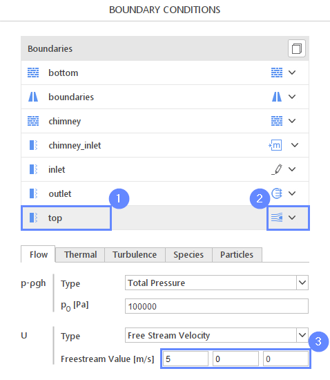
39. Boundary Conditions - Top
For the top boundary, we will use the same Free Stream condition as for the inlet.
- Select top boundary
- Set the Free Stream character
- Define free stream velocity:
U Freestream Value \({\sf [m/s]}\)500
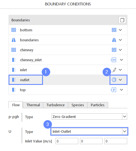
40. Boundary Conditions - Outlet
At the outlet, we will apply an Outflow boundary condition. To prevent reverse flow, we will set an Inlet-Outlet condition that behaves like a zero gradient when air is escaping, and it blocks the reverse flow by imposing zero velocity when entering the domain.
- Select outlet
- Set the Outflow character
- Change velocity type
U TypeInlet-Outlet
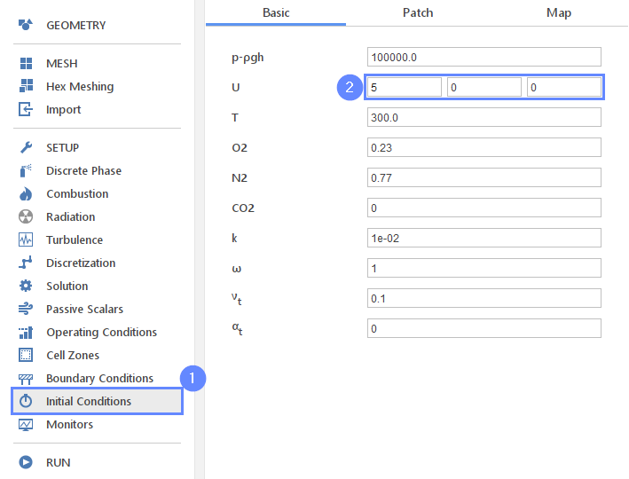
41. Initial Conditions
At the initial state, we assume a constant velocity on the domain filled by the air.
- Go to Initial Conditions panel
- Set the initial velocity
U500
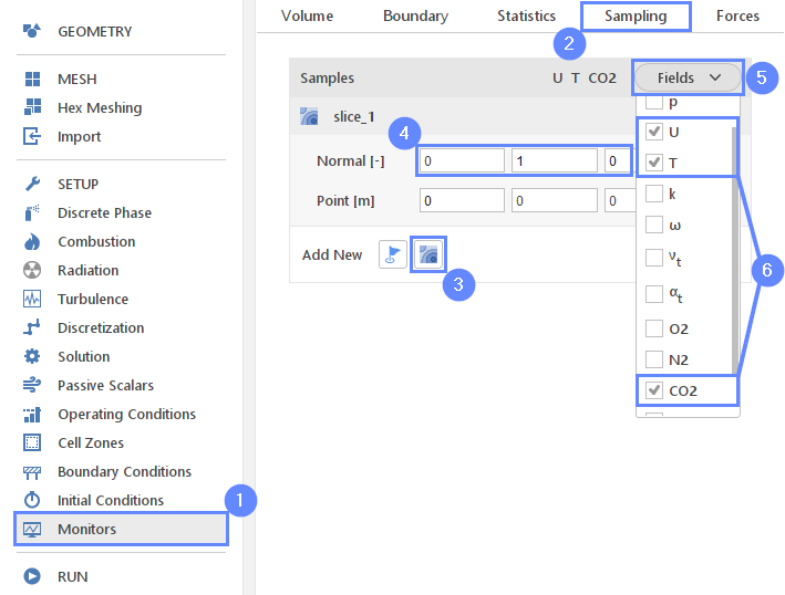
42. Monitors – Sampling
During calculation, we can observe intermediate results on a section plane. To sample data on a plane, we need to define the plane and also select fields that will be sampled. Note, runtime post-processing can only be configured before starting calculations and cannot be changed later on.
- Go to Monitors panel
- Switch to Sampling tab
- Select Create Slice
- Set slice plane normal vector
Normal \({\sf [-]}\)010 - Expand Fields list
- Select velocity U, temperature T and phase CO2
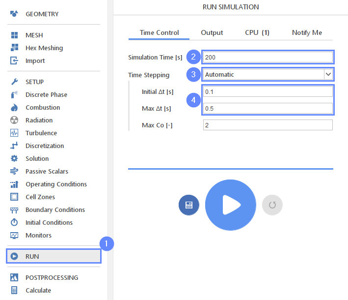
43. Run - Time Control
In any simulation, it is often convenient to allow the solver to automatically determine the appropriate time step. To use this option, we need to define time step constraints by specifying the initial time step, which the solver can adjust during computations, and the maximum time step value. All other parameters can be left at their default settings.
- Go to RUN panel
- Set the Simulation Time [s] to 200
- Change Time Stepping to Automatic
- Set initial and maximum timesteps (solver will start computation with the initial value and adjust it in the next iterations not exceeding the maximum value)
Initial \(\Delta t\) \({\sf [s]}\)0.1
Max \(\Delta t\) \({\sf [s]}\)0.5
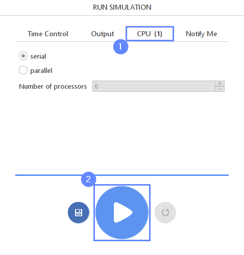
44. Run - CPU
To speed up the calculation process, take advantage of parallel computing and increase the number of CPUs based on your PC’s capability. The free version allows you to use only one processor (serial mode). To get the full version, you can use the contact form to Request 30-day Trial
Estimated computation time for serial mode: 40 minutes
- Switch to CPU tab
- Click Run Simulation button
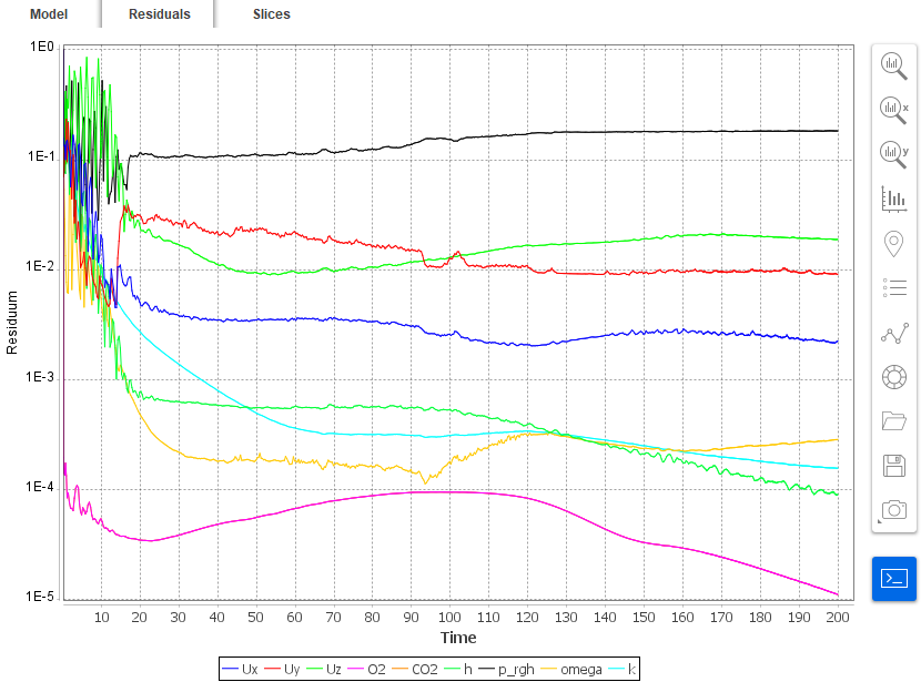
45. Residuals
When the calculation is finished, we should see a similar residual plot.
- Go to Residuals tab
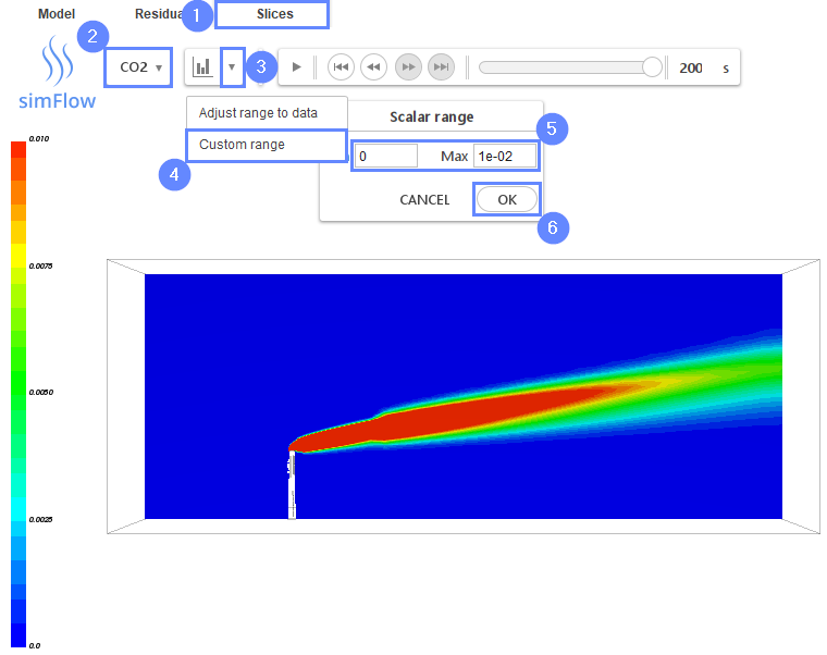
46. Slice - CO2 Field
Slices tab appears next to the Residuals . Under this tab, we can preview results on the defined section plane.
The Slices tab appears next to the Residuals tab. In this section, we will display the CO2 concentration on a defined section plane. We will also adjust the color range to make it easier to visualize regions with low CO2 concentrations, allowing for a more detailed analysis of the dispersion.
- Change tab to Slices
- Select the phase CO2
- Expand data range options
- Select Custom Range
- Provide the range to Min0 and Max0.01
- Click OK
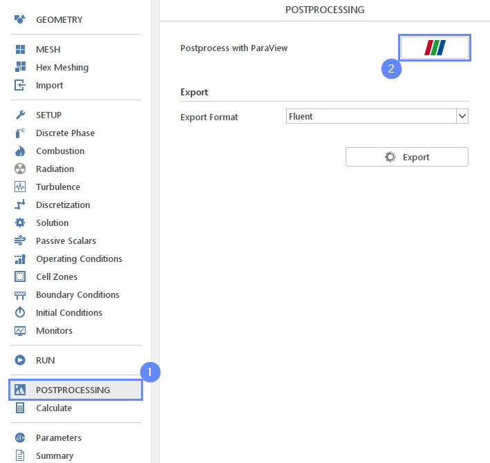
47. Postprocessing - ParaView
Once the computations have been completed, we can perform advanced visualization of the results using ParaView.
- Go to POSTPROCESSING panel
- Click on Run ParaView
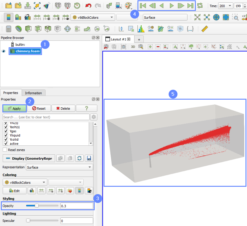
48. ParaView - Load Results
Load the results into the program.
- Make sure you have your case selected chimney.foam
- Click Apply to load results
- Reduce the opacity to 0.3
- Select coloring variable to vtkBlocksColors
- Play the animation using Play button
- Results will be shown in the 3D graphic window
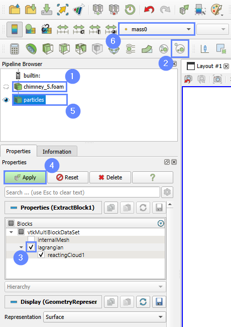
49. ParaView - Extract Particles Block
In order to display the particles in a different scheme, it is necessary to first extract them from the overall results.
- Select baseline results chimney.foam
- Select Extract Block
- Check lagrangian group
- Confirm with the Apply button
- Double-click on its name and rename it to particles
- Select coloring variable to mass0
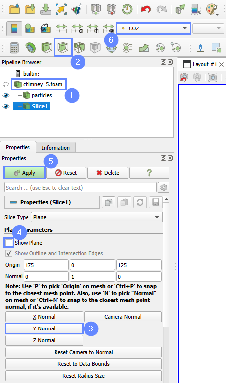
50. ParaView - Slice
We will create the cross-section through the computational domain to display the CO2 distribution.
- Select the chimney.foam from Pipeline Browser
- Select Slice
- Set the plane normal along Y axis using Y Normal button
- Uncheck Show Plane
- Press Apply
- From the drop-down coloring menu select CO2
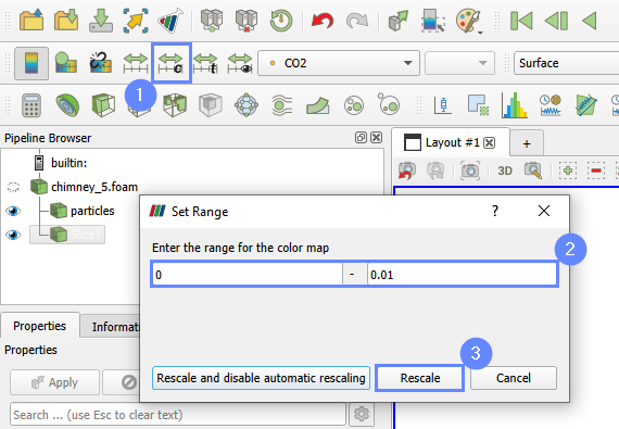
51. ParaView - Rescale
Scale the CO2 results to get a range of up to 1% carbon dioxide contribution.
- Click on Rescale to Custom Data Range
- Set the range from 0 to 0.01
- Confirm by clicking Rescale
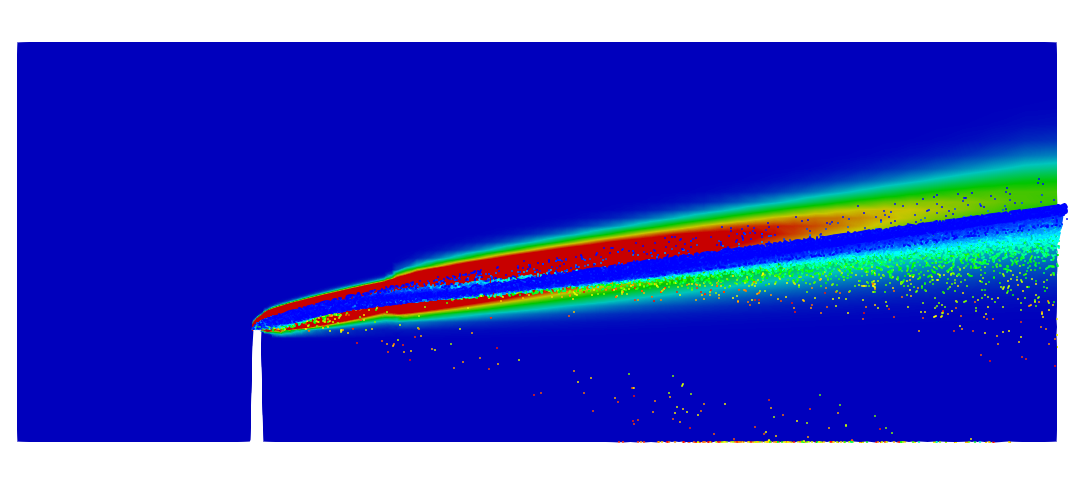
52. ParaView - Results
Orient the view parallel the XZ plane and play with animation buttons to investigate the time history of the flow.