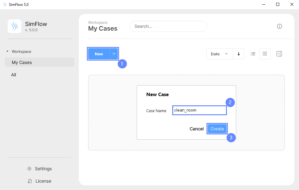
2. Create Case
Open SimFlow and create a new case named clean room
- Click New
- Provide name clean room
- Click Create to open a new case
3. Import Geometry
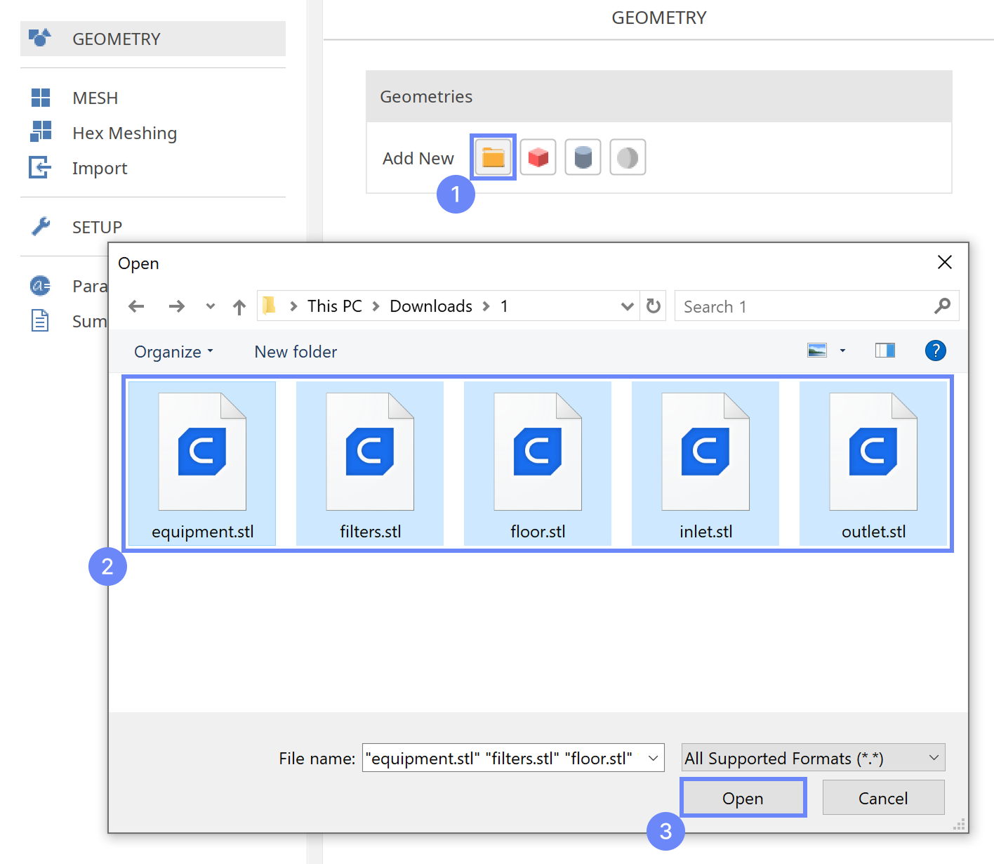
4. Import Geometry II
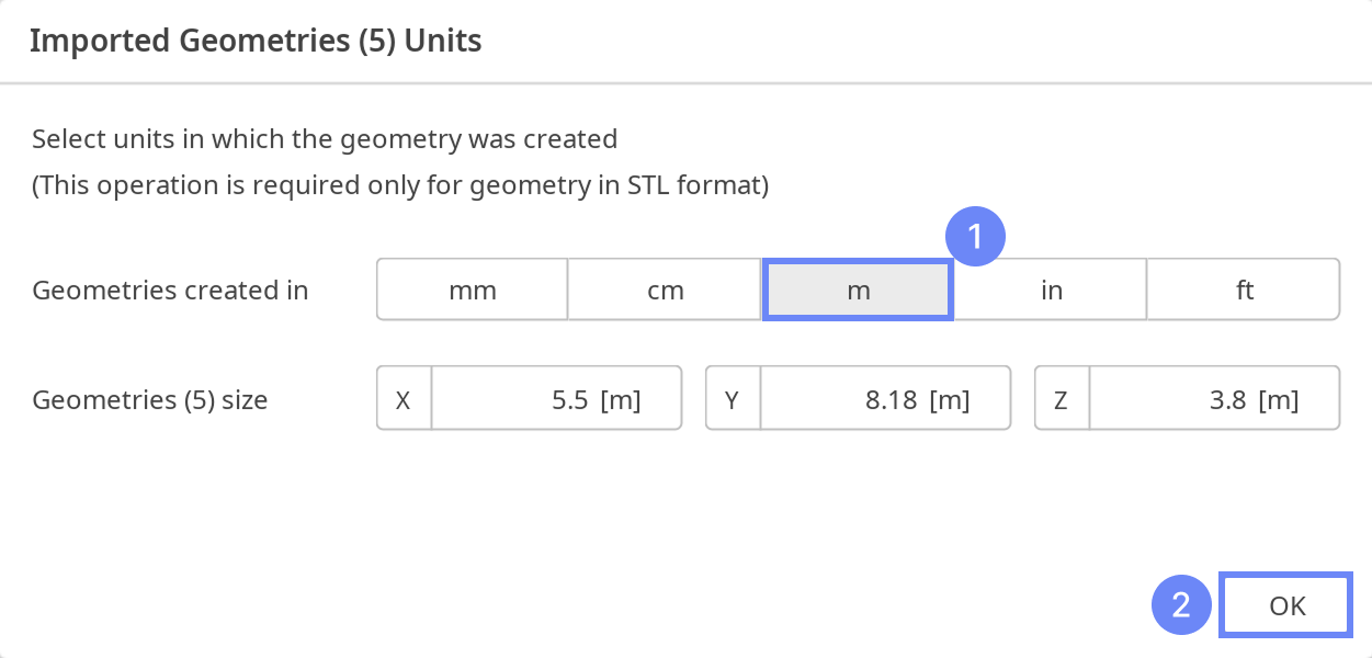
If the imported geometry is in STL format, be aware that STL files do not include unit information. Therefore, you must manually specify the correct unit after import. If you’re unsure of the original unit used during export, you can estimate it by checking the Geometry size displayed in the interface.
In this case, since the fan geometry is correctly defined in meters, no rescaling is required.
- Ensure STL geometry units are set to meter
- Click OK
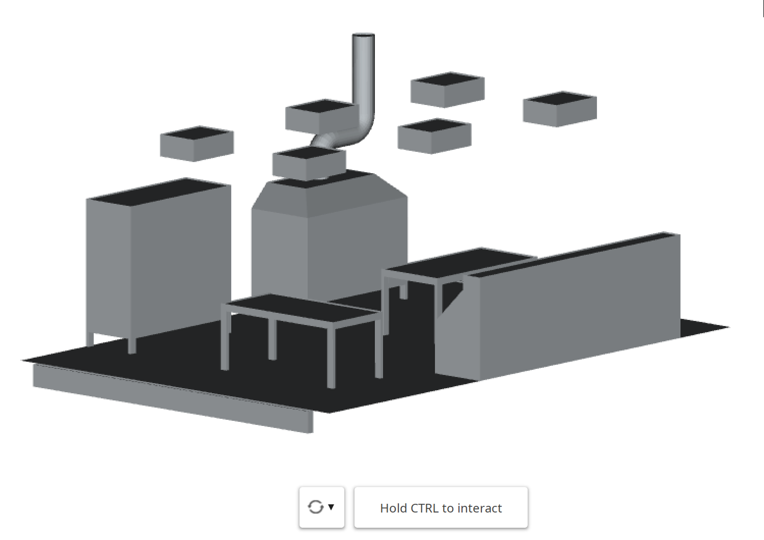
5. Geometry - Clean Room
After importing the geometry, it will appear in the 3D window. The geometry components include:
- Cleanroom furniture (equipment)
- Ventilation inlets
- Ventilation outlets
- Floor – 2D surface
The walls of the cleanroom are not included, as they will be defined by the base mesh in later steps.
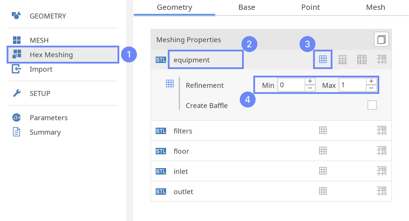
6. Meshing Parameters - Clean Room Equipment
To create the mesh, we need to specify the meshing options for the given geometries.
For the equipment inside the room, we will refine the mesh.
- Go to Hex Meshing panel
- Select the equipment component
- Enable Mesh Geometry for equipment
- Set Refinement to
Min 0
Max 1
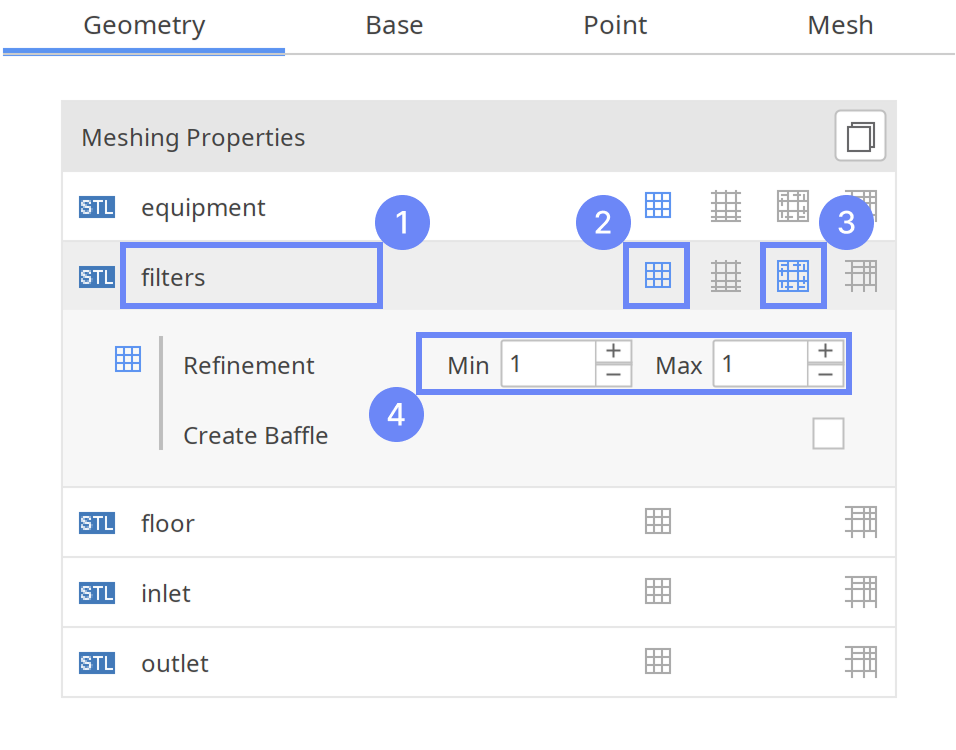
7. Meshing Parameters - Filters
For the filters, we will also refine the mesh. Since the filters are modeled as a porous medium, we need to create a dedicated cell zone for them. This will allow us to apply the porous media model and accurately represent the flow resistance introduced by the filter.
- Select the filters component
- Enable Mesh Geometry
- Enable Create Cell Zone
- Set Refinement to
Min 1
Max 1
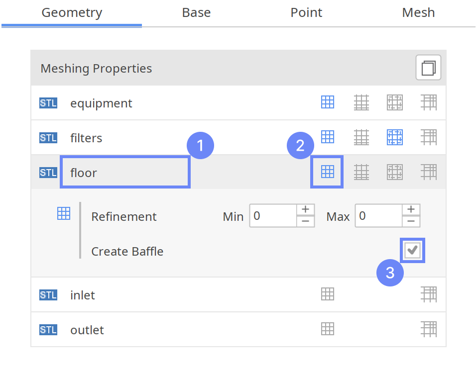
8. Meshing Parameters - Floor
In this simulation, we want to model a suspended floor on which equipment is placed, with open space below for air to be discharged. Since a floor is permeable but includes filters and ventilation grilles resist airflow, we will again use a porous medium. In this case, the floor thickness is very small, so we can model it as a 2D surface. The porosity will be defined later using the Porous Baffle boundary condition.
To model the floor by the surface inside the domain (immersed boundary), make sure to enable the Create Baffle option. A baffle is a thin internal surface that separates regions without adding physical thickness. It is commonly used for internal walls, fans, or porous surfaces. By duplicating the original surface, the baffle creates two coincident faces, allowing different boundary conditions to be applied on each side (immersed boundary approach).
- Select the floor component
- Enable Mesh Geometry
- Mark Create Baffle
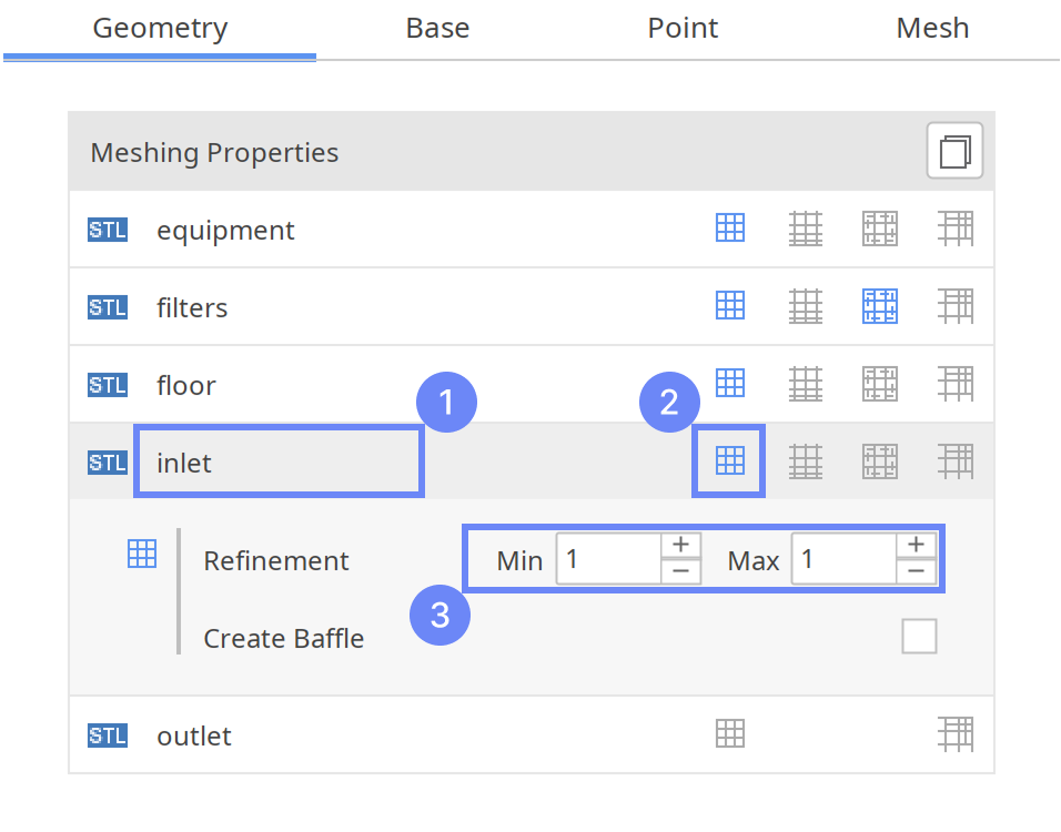
9. Meshing Parameters - Inlet
For the inlet and outlet, apply mesh refinement near its surface to level 1, ensuring accurate resolution of airflow entering and leaving the cleanroom.
- Select the inlet component
- Enable Mesh Geometry
- Set Refinement to
Min 1
Max 1
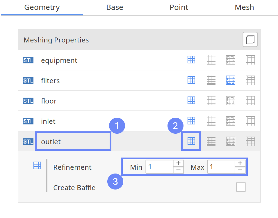
10. Meshing Parameters - Outlets
Repeat the same setup for the outlet.
- Select the outlet component
- Enable Mesh Geometry
- Set Refinement to
Min 1
Max 1
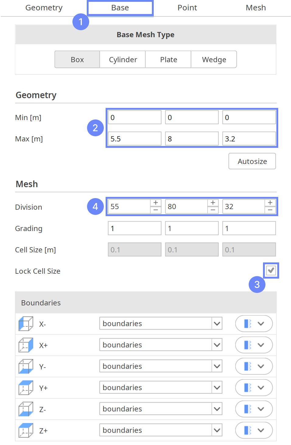
11. Base Mesh - Domain
To define the cleanroom boundaries, we will use the Box base mesh type. It matches the rectangular shape of the room.
- Go to Base tab
- Set the base mesh size:
Min \({\sf [m]}\)000
Min \({\sf [m]}\)5.583.2 - Mark Lock Cell Size
- Define the number of divisions along one axis — the remaining directions will adjust automatically
Division558032
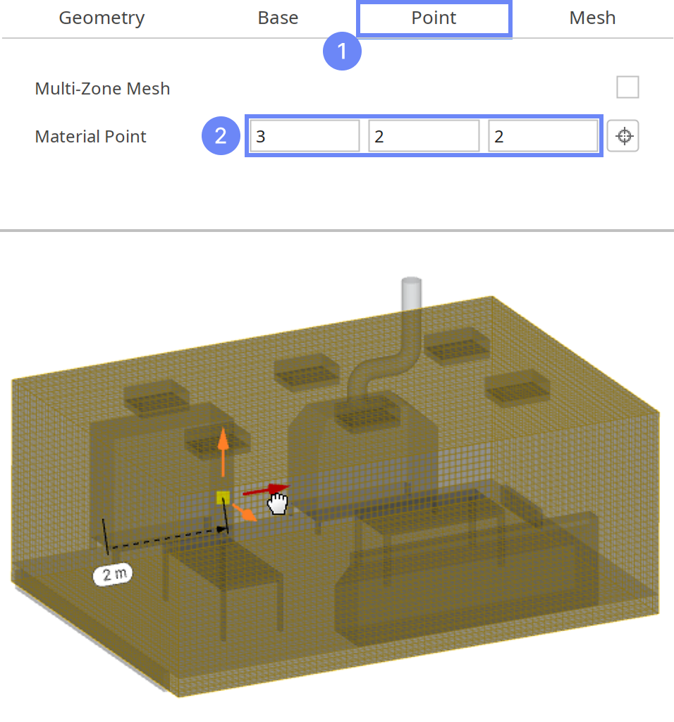
12. Material Point
The material point indicates which side of the geometry the mesh will be retained on. Since we are simulating airflow inside the clean room, the material point must be placed within the base mesh and outside the equipment.
- Go to Point tab
- Specify location inside clean room
Material Point322
You can specify the point location directly in the 3D view. Hold the CTRL key and drag the arrows to move the point to the desired location.
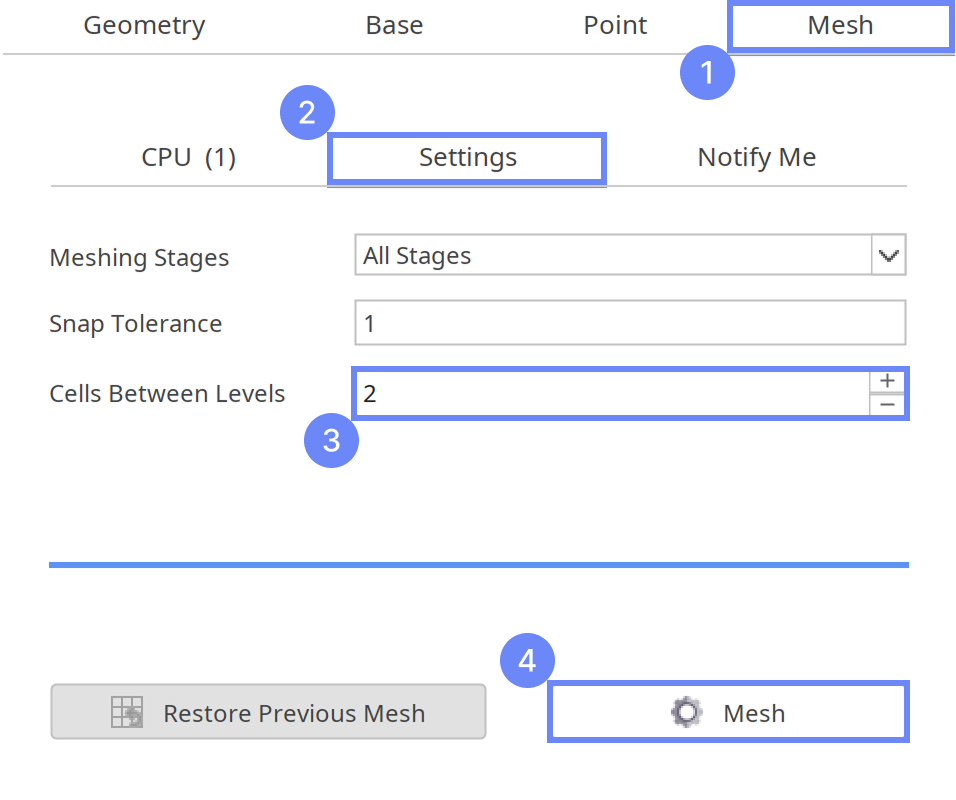
13. Start Meshing
In this step, we will initiate the meshing process.
In the meshing panel, you can indicate how many CPUs you would like to use for this process. Note that if you are using the free version of SimFlow, you may only use serial meshing and cannot create meshes larger than 200,000 nodes.
To meet this limit, we need to reduce the cell count by decreasing the number of cells between refinement levels.
If you would like to test full version Request 30-day Trial
- Switch to Mesh tab
- Go to Settings
- Set Cells Between Levels to 2
- Start the meshing process with Mesh button
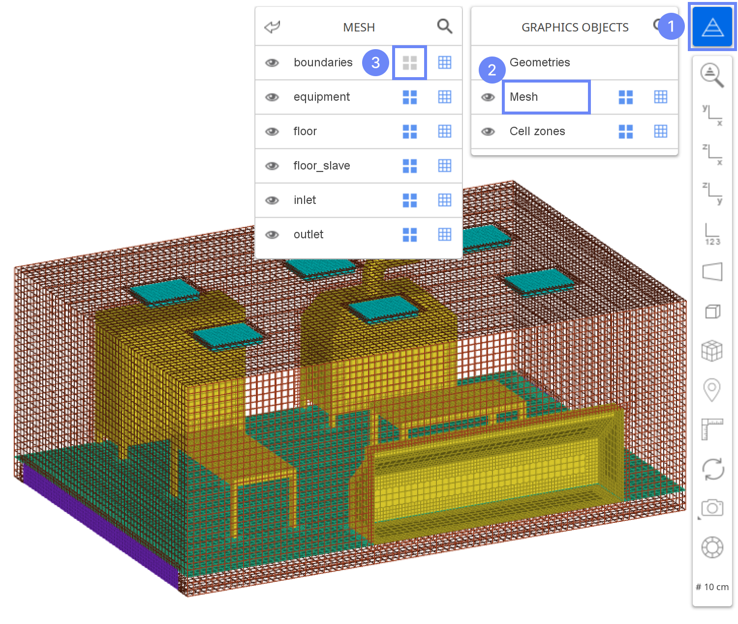
14. Mesh
After the meshing process is complete, the mesh will appear on the screen.
To preview the mesh resolution and internal boundaries of the cleanroom, we can hide the external boundary faces while keeping the edges and remaining internal boundaries visible.
- Expand the Graphics Objects List
- Go to MESH
- Hide mesh faces for the boundaries
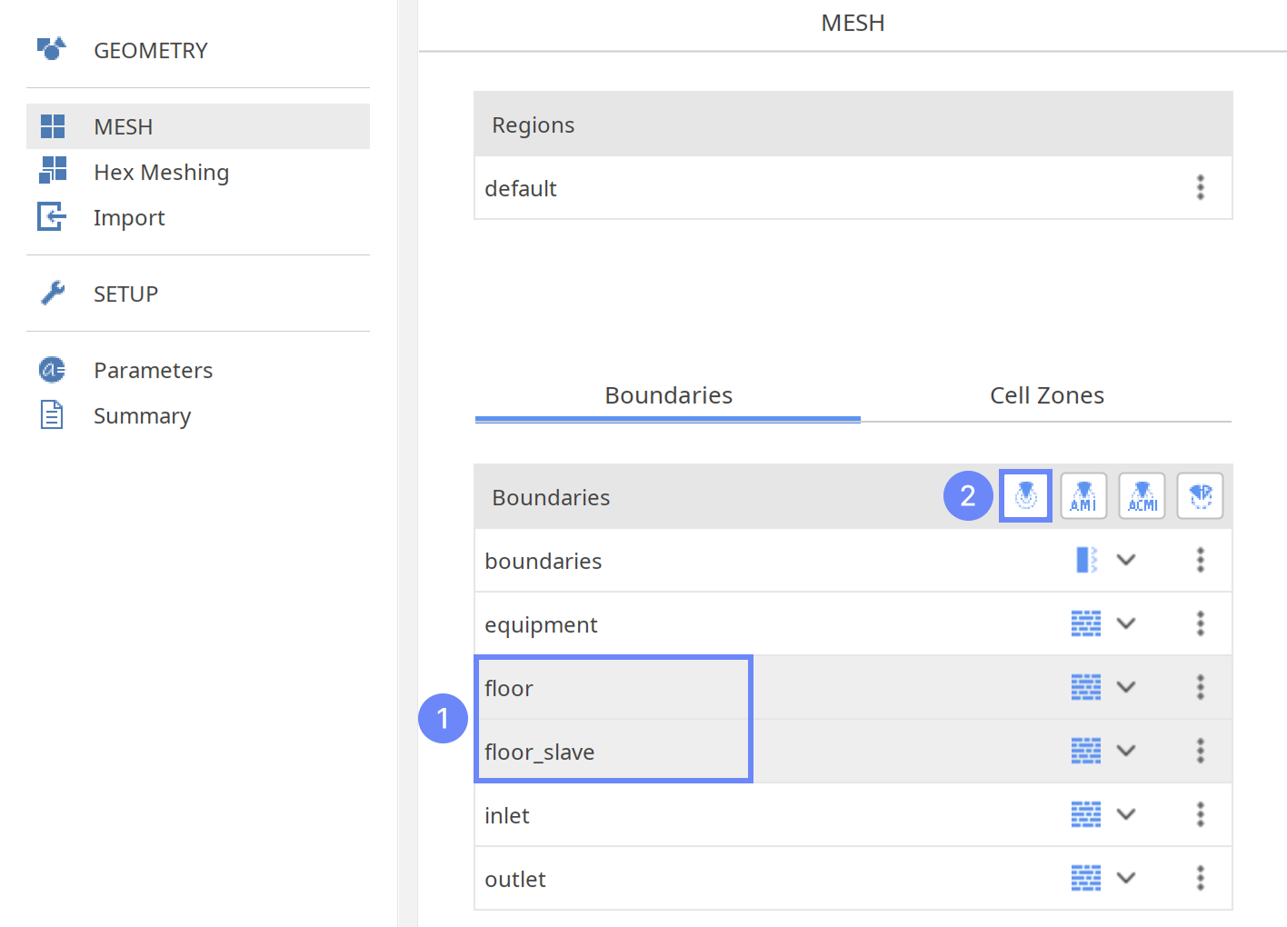
15. Create Floor Interface
In the mesh setup, we enabled baffle creation for the floor, which splits the mesh along the surface Now, we will create a Cyclic Interface to connect both sides of the internal boundary, allowing airflow through the floor.
- Holding Ctrl key select following boundaries
floor
floor_slave - Select Create Cyclic Interface
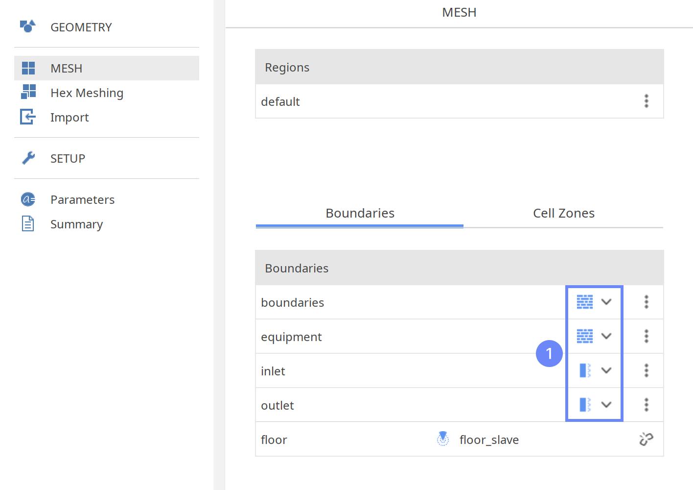
16. Check Mesh Boundaries
Review the boundary list and assign appropriate types to each boundary. Wall type prevents fluid from crossing, while Patch type allows fluid to pass through, making it suitable for inlets and outlets.
- Define boundary types accordingly
boundaries wall
equipment wall
inlet patch
outlet patch
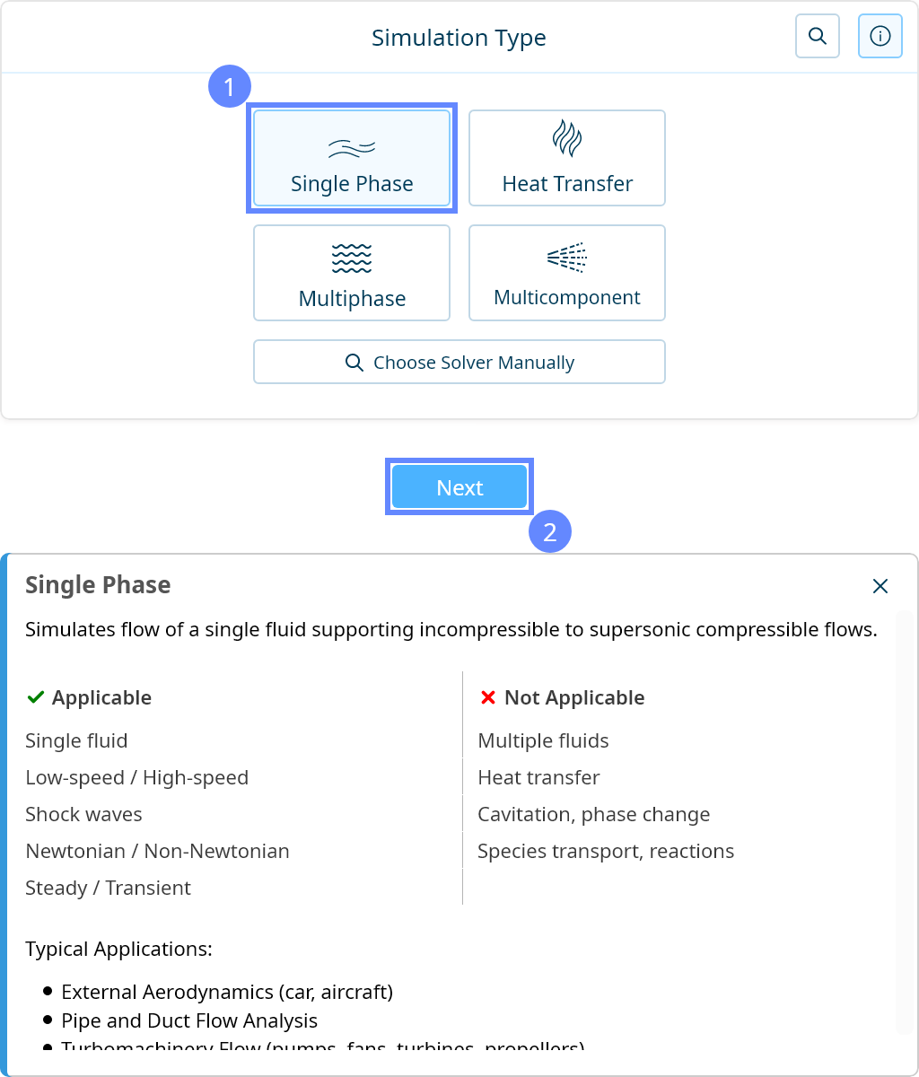
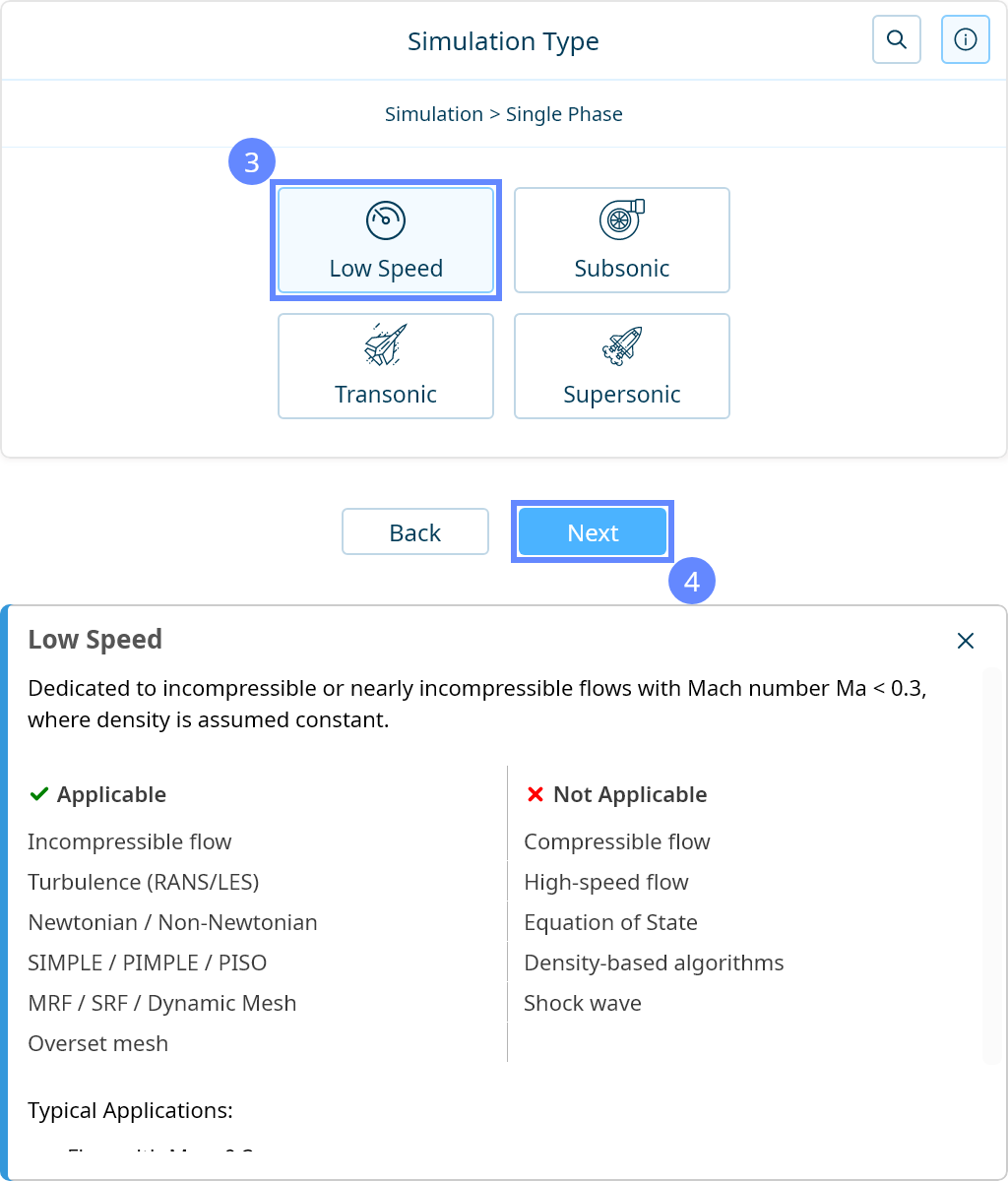
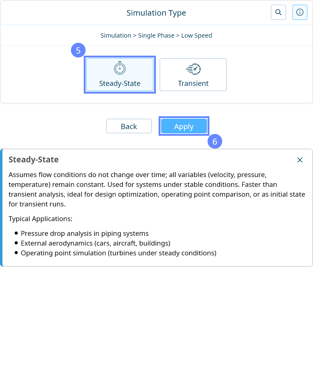
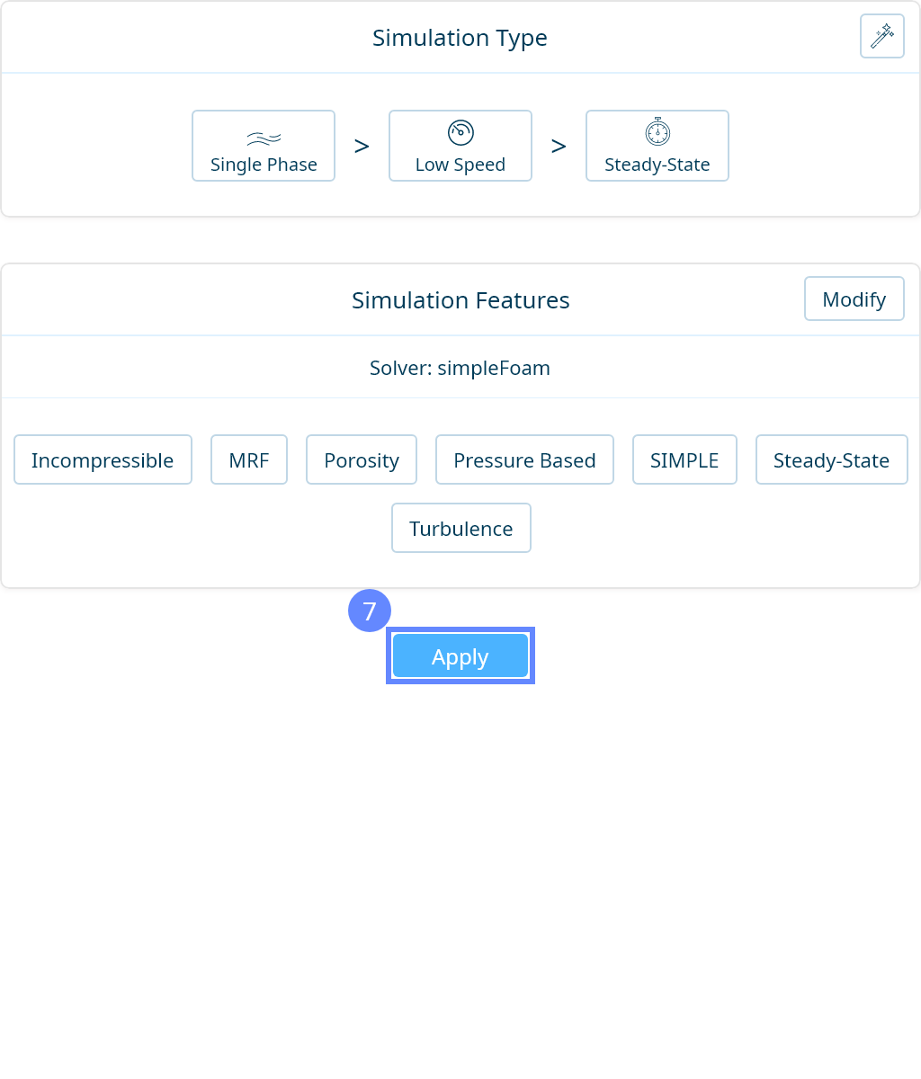
17. Simulation Type
Cleanroom simulations can be performed as transient analyses, capturing the full flow history. However, such calculations are typically very time-consuming. In this tutorial, we will show an alternative approach to measure air residence time using a steady-state simulation with a passive scalar model.
For this purpose, we will use a single-phase, steady-state simulation of incompressible turbulent flow.

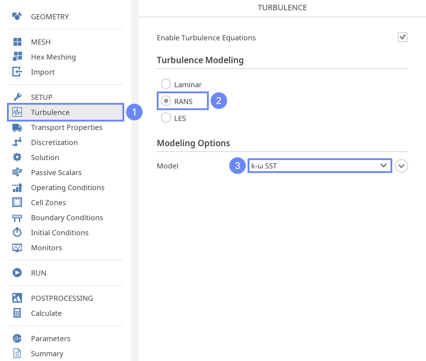
18. Turbulence
We are going to use the standard \(k{-}\omega \; SST\) model to resolve turbulence.
- Go to Turbulence panel
- Select RANS modeling
- Select \(k{-}\omega \; SST\) model
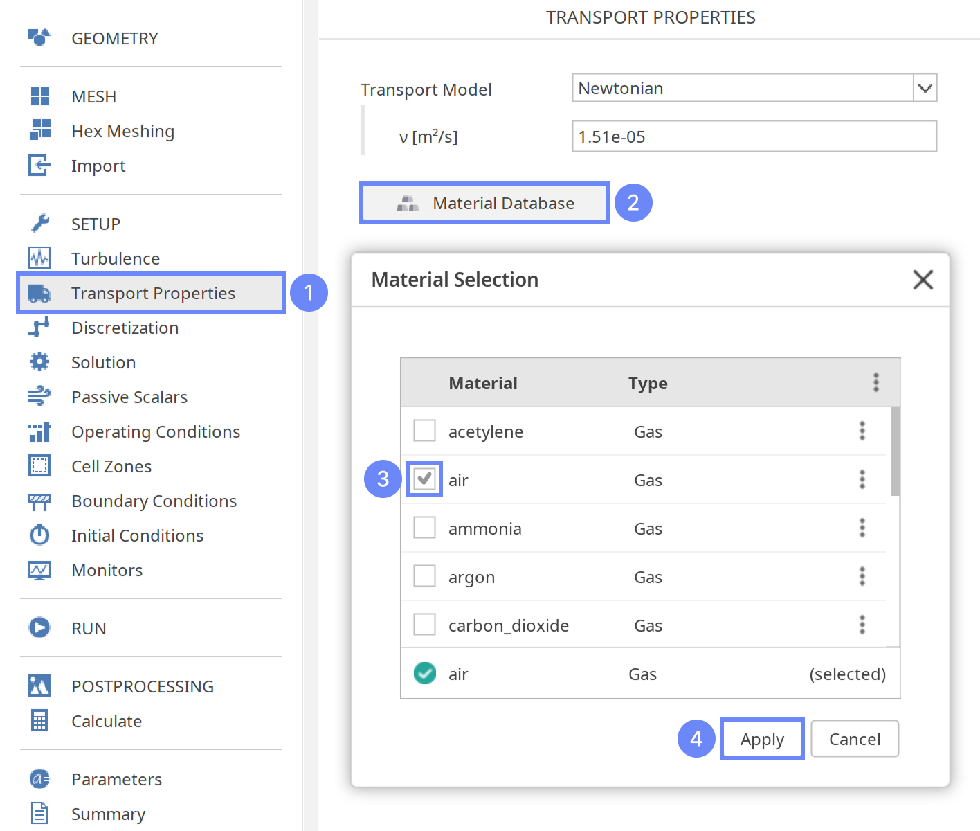
19. Transport Properties - Air
As a fluid material, we will use air.
- Go to Transport Properties panel
- Open Material Database
- Select air from the list
- Click Apply
Selecting material from the Material Database will fill all inputs in the Transport Properties panel. We are still able to overwrite these values at any time.
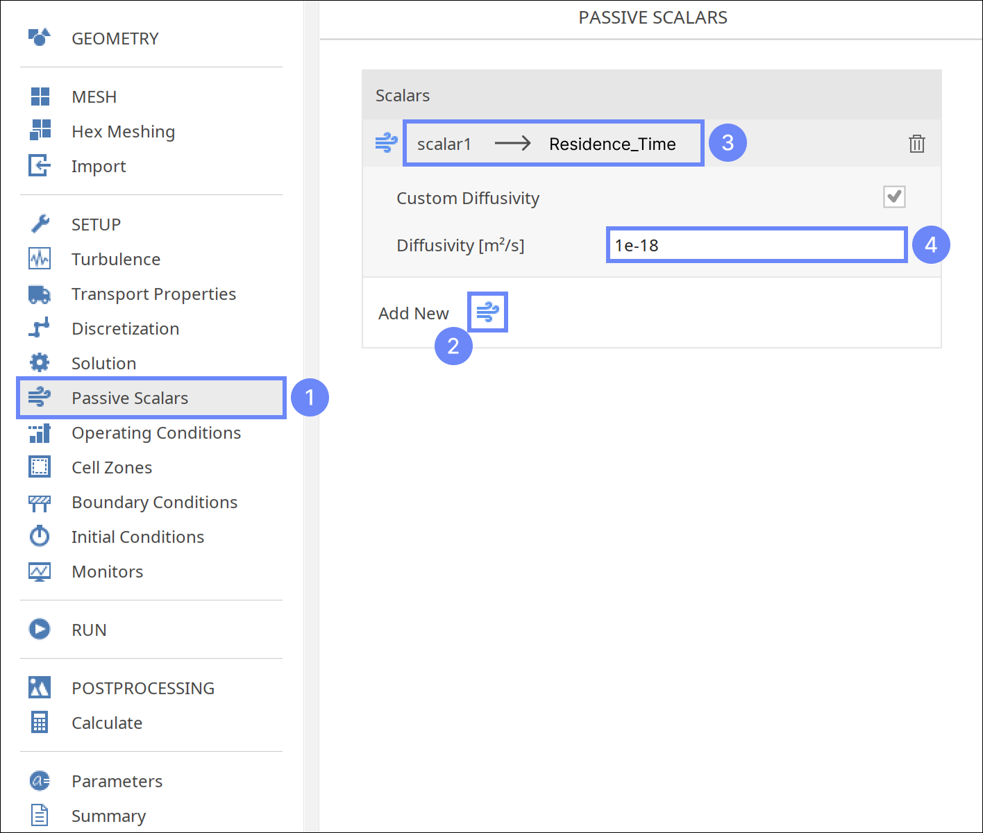
21. Residence Time - Passive Scalar
Now, we will create a passive scalar representing Residence Time and assign it a negligible diffusivity.
- Go to Passive Scalars panel
- Press Add new passive scalar Equations button
- Change scalar name (double-click on a scalar name to start editing)
scalar1 → Residence Time - Set the diffusivity
Diffusivity \({\sf [m^2/s]}\)1e-18
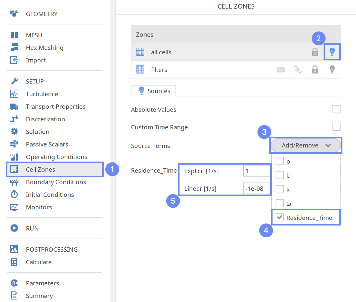
22. Residence Time - Source Term
In the Cell Zone panel, we will define the source term for the Residence Time field. In each cell, the fluid residence time will increase at a constant rate of 1 per second.
Additionally, we will add an implicit source to limit the maximum value of the residence time to 1e8 s. Beyond this threshold, the residence time will no longer increase, effectively acting as an upper limit.
- Go to Cell Zones panel
- Mark Source Term for all cells
- Expand Add/Remove fields
- Select the Residence_Time
- Specify the source rate
Residence_Time Explicit \({\sf [1/s]}\)1
Residence_Time Linear \({\sf [1/s]}\)-1e-8
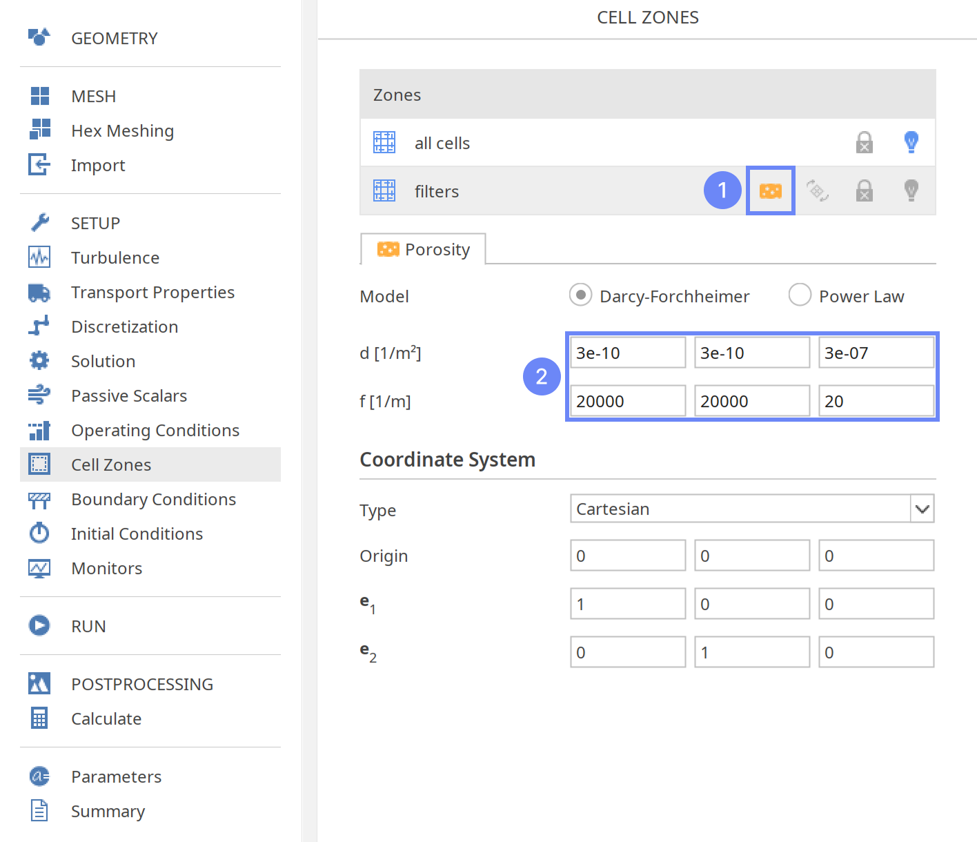
23. Porous Media - Filters
Now, we will apply porosity to the previously created cell zone to model the HEPA filters located after the inlet.
- Check Porous Zone for the filters cell zone
- Use a default Darcy-Forchheimer model and set its parameters accordingly
d \({\sf [\frac{1}{m^2}]}\)3e-103e-103e-7
f \({\sf [\frac{1}{m}]}\)200002000020
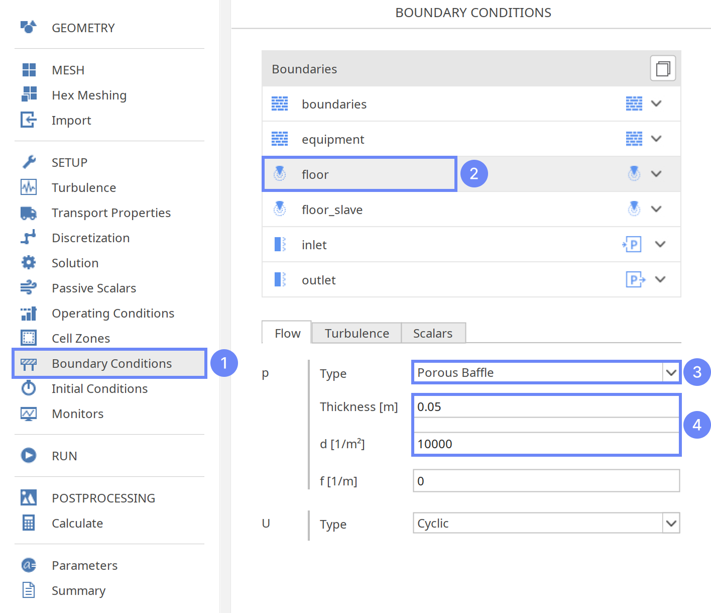
24. Boundary Conditions - Floor
We will now specify the model’s boundary conditions.
To model the permeable floor, we will apply Porous Baffle boundary conditions to the floor interface.
- Go to Boundary Conditions panel
- Select floor boundary
- Change the pressure condition to Porous Baffle
- Define its parameter accordingly
Thickness \({\sf [m]}\)0.05
d \({\sf [\frac{1}{m^2}]}\)10000
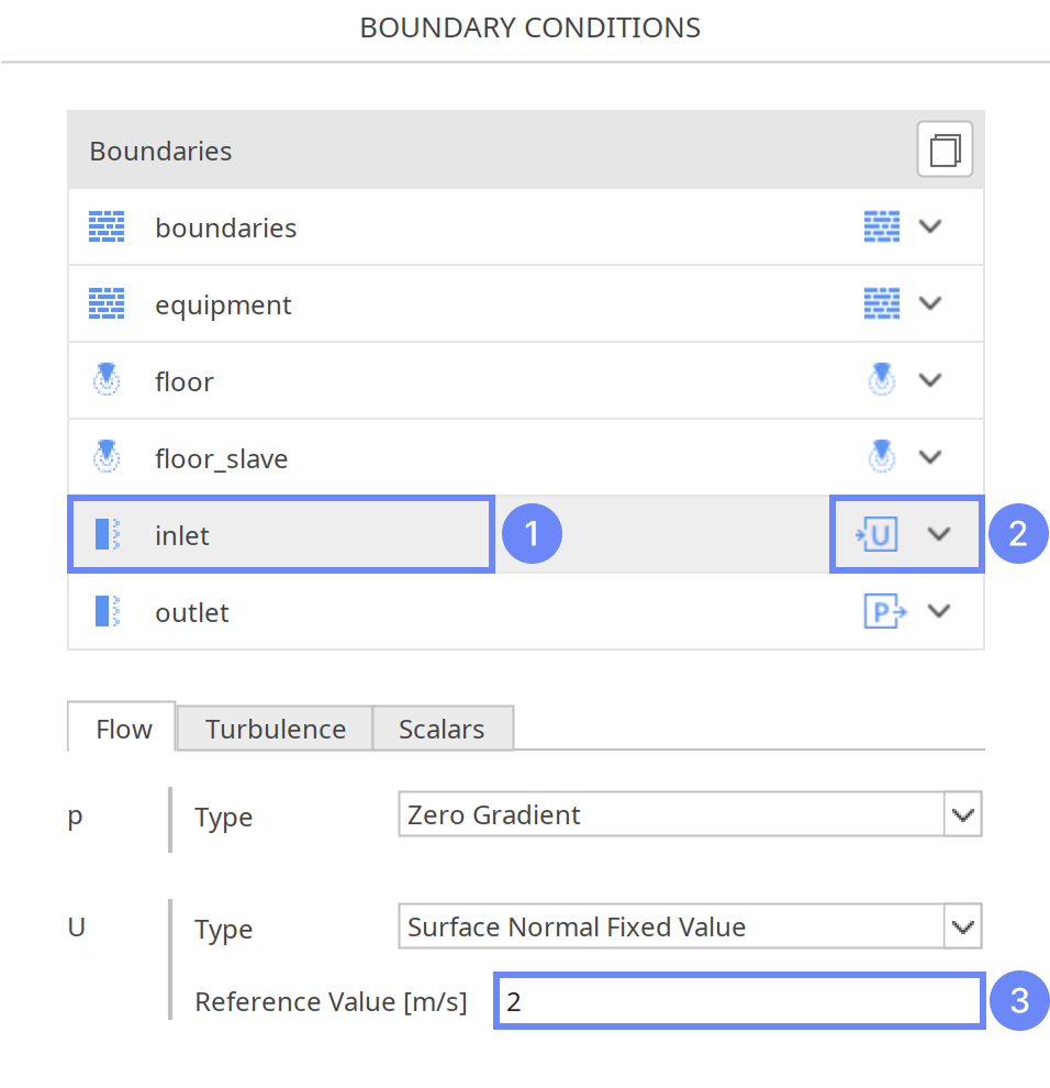
25. Boundary Conditions - Inlet
To model the ventilation inlet, we will set the constant velocity using Velocity Inlet preset.
- Select inlet boundary
- Set the Velocity Inlet preset
- Set the surface normal velocity
U Reference Value \({\sf [m/s]}\)2
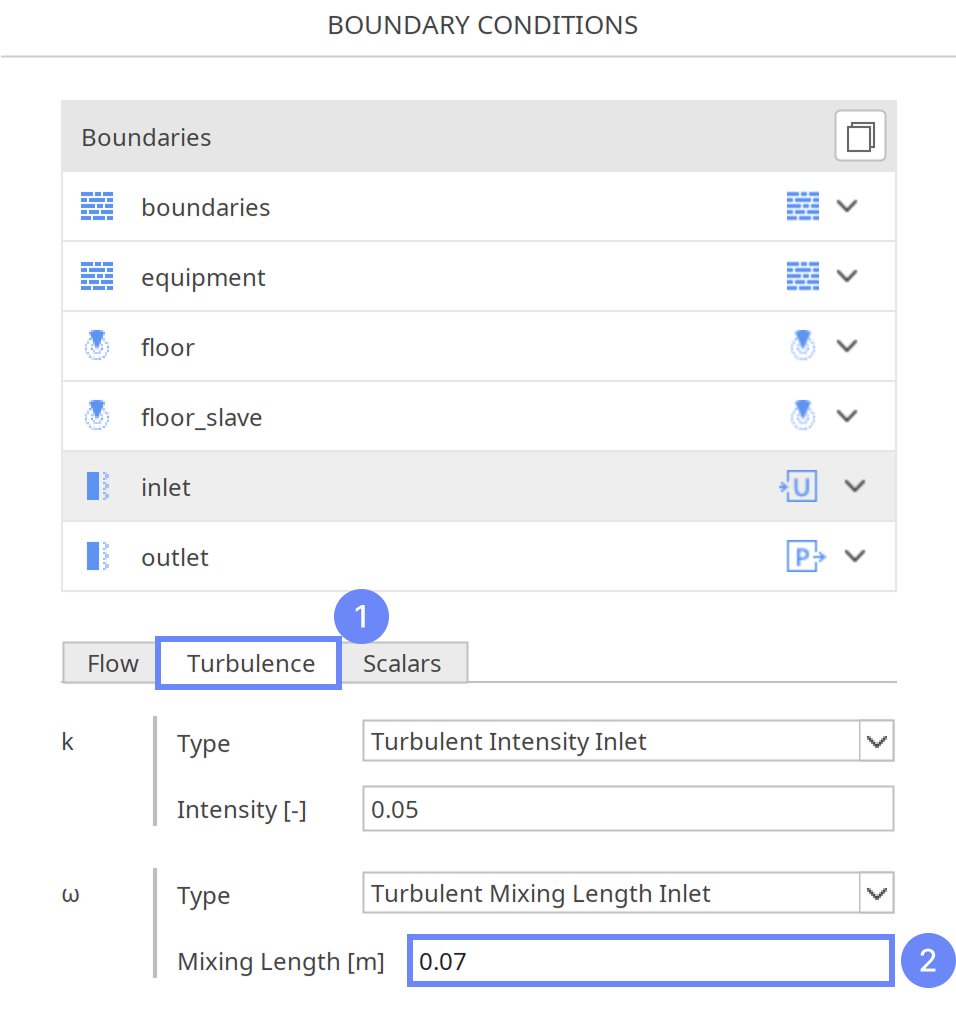
26. Boundary Conditions - Inlet - Turbulence
We will also update the turbulent mixing length at the inlet.
- Switch to Turbulence tab
- Set the value
\(\omega\) Mixing Length \({\sf [m]}\)0.07
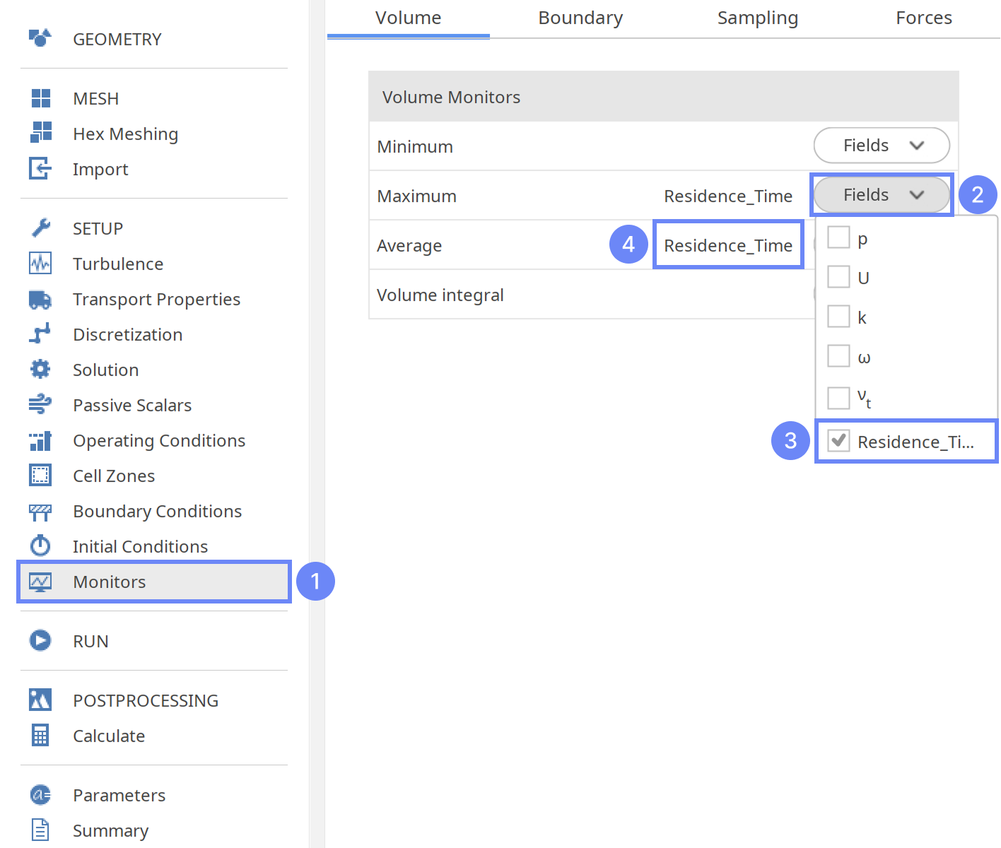
27. Monitors - Volume Monitors
During the calculation, we can track fluid parameters or observe intermediate results using section planes or probe plots. Note that runtime post-processing must be defined before starting the calculations and cannot be modified afterward.
Firstly, we will define volume monitor to track maximum and average residence time in the clean room.
- Go to Monitors panel
- Expand Fields list for Maximum volume monitor
- Mark Residence Time
- Repeat this step for the Average volume monitor
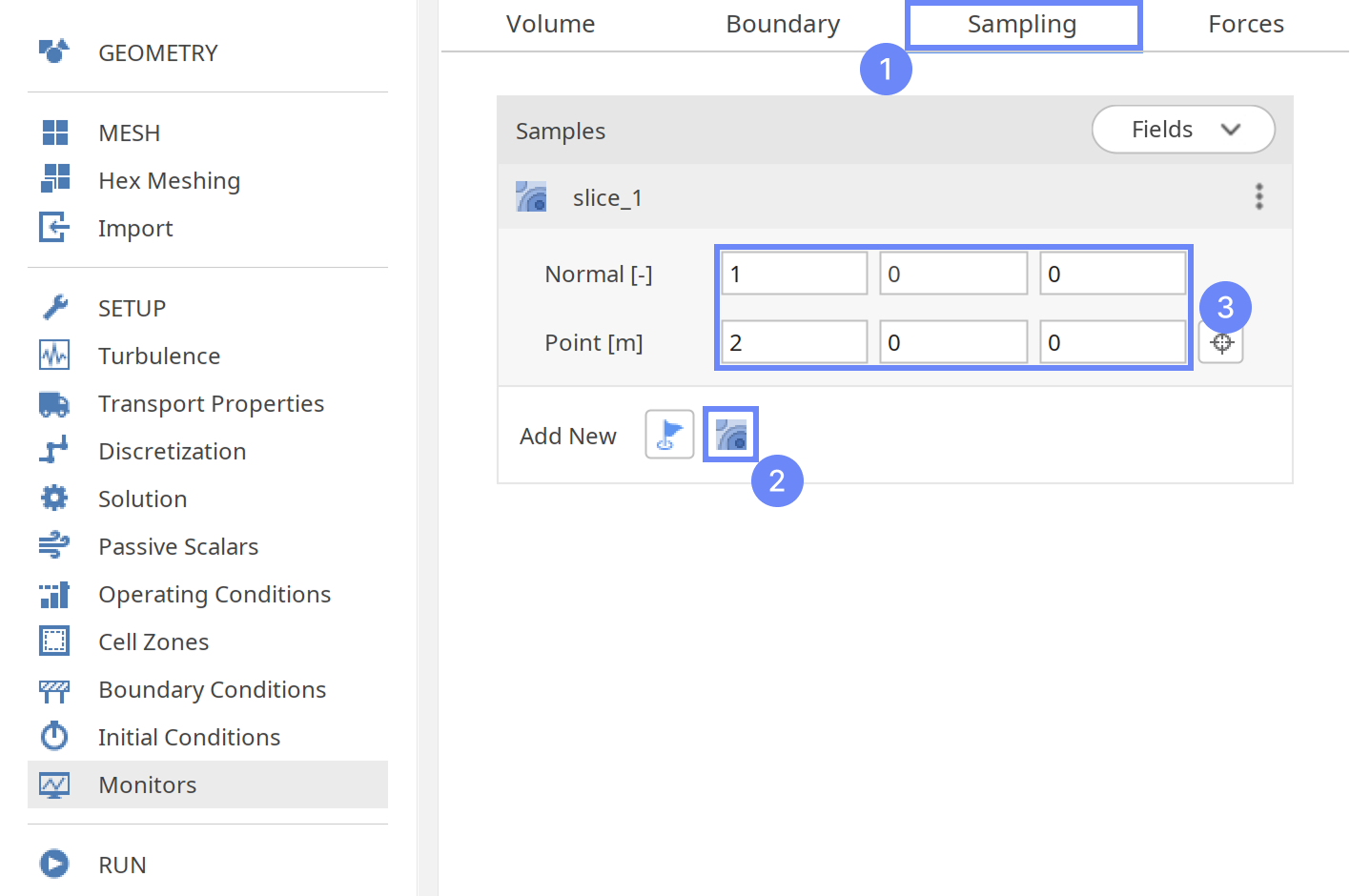
28. Monitors - Create Slice (I)
Now, we will create two slices to preview the field map across the domain.
- Switch to Sampling tab
- Select Create Slice
- Set slice plane normal vector and its point
Normal \({\sf [-]}\)100
Point \({\sf [m]}\)200
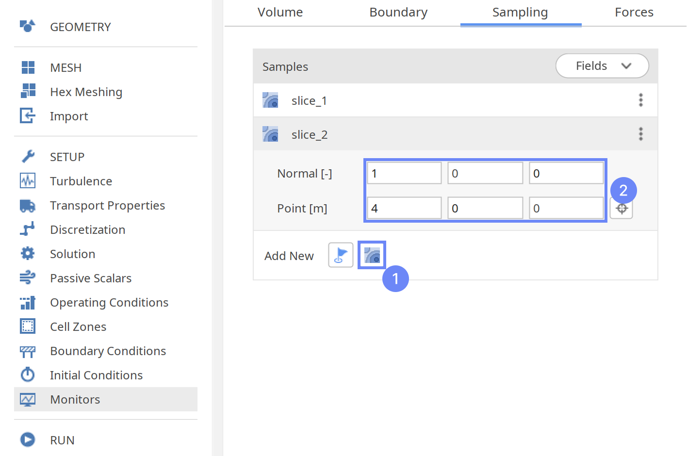
29. Monitors - Create Slice (II)
Create the second slice.
- Select Create Slice
- Set slice plane normal vector and its point
Normal \({\sf [-]}\)100
Point \({\sf [m]}\)400
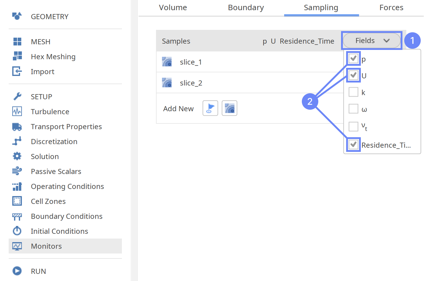
30. Monitors – Sampling (III)
Now, we need to specify the variables to be sampled.
- Expand Fields list
- Select the following parameters
pressure p
velocity U
Residence Time Residence Ti…
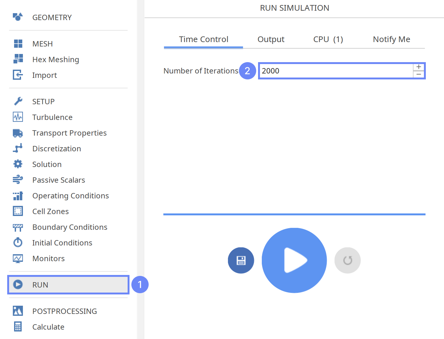
31. Run - Time Control
Finally, we can start our computation.
- Go to RUN panel
- Set the maximal Numbers of Iterations to 2000
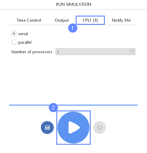
32. Run - CPU
To speed up the calculation process, take advantage of parallel computing and increase the number of CPUs based on your PC’s capability. The free version allows you to use only one processor (serial mode). To get the full version, you can use the contact form to Request 30-day Trial
Estimated computation time for serial mode: 10 minutes
- Switch to CPU tab
- Click Run Simulation button
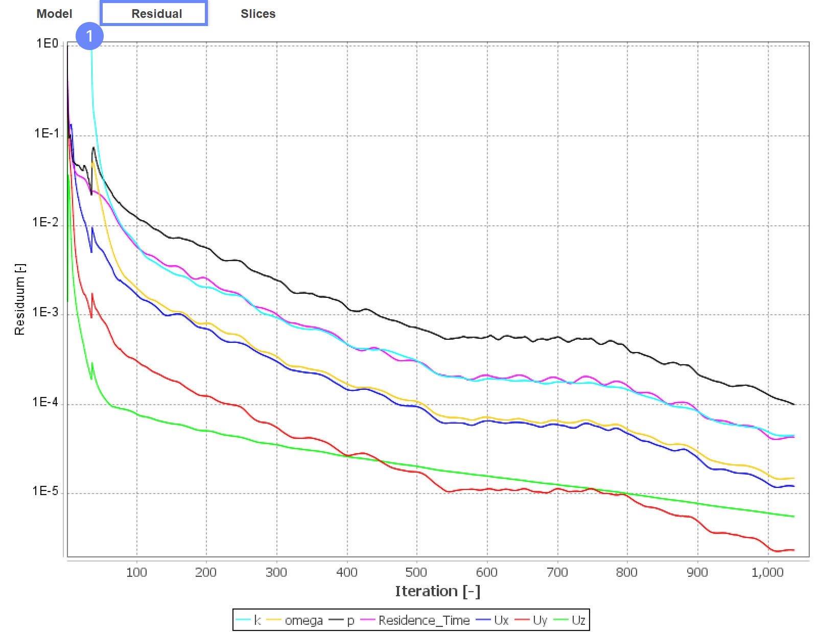
33. Residuals
When the calculation is finished, we should see a similar residual plot. All the residual values have reached \(10^{-4}\) and the solver has automatically stopped the calculation. The residuals are the measure of how results change between iteration. Reaching a very low value indicates that we have found a steady-state solution and results do not change regardless of further computations.
- Preview the Residuals tab
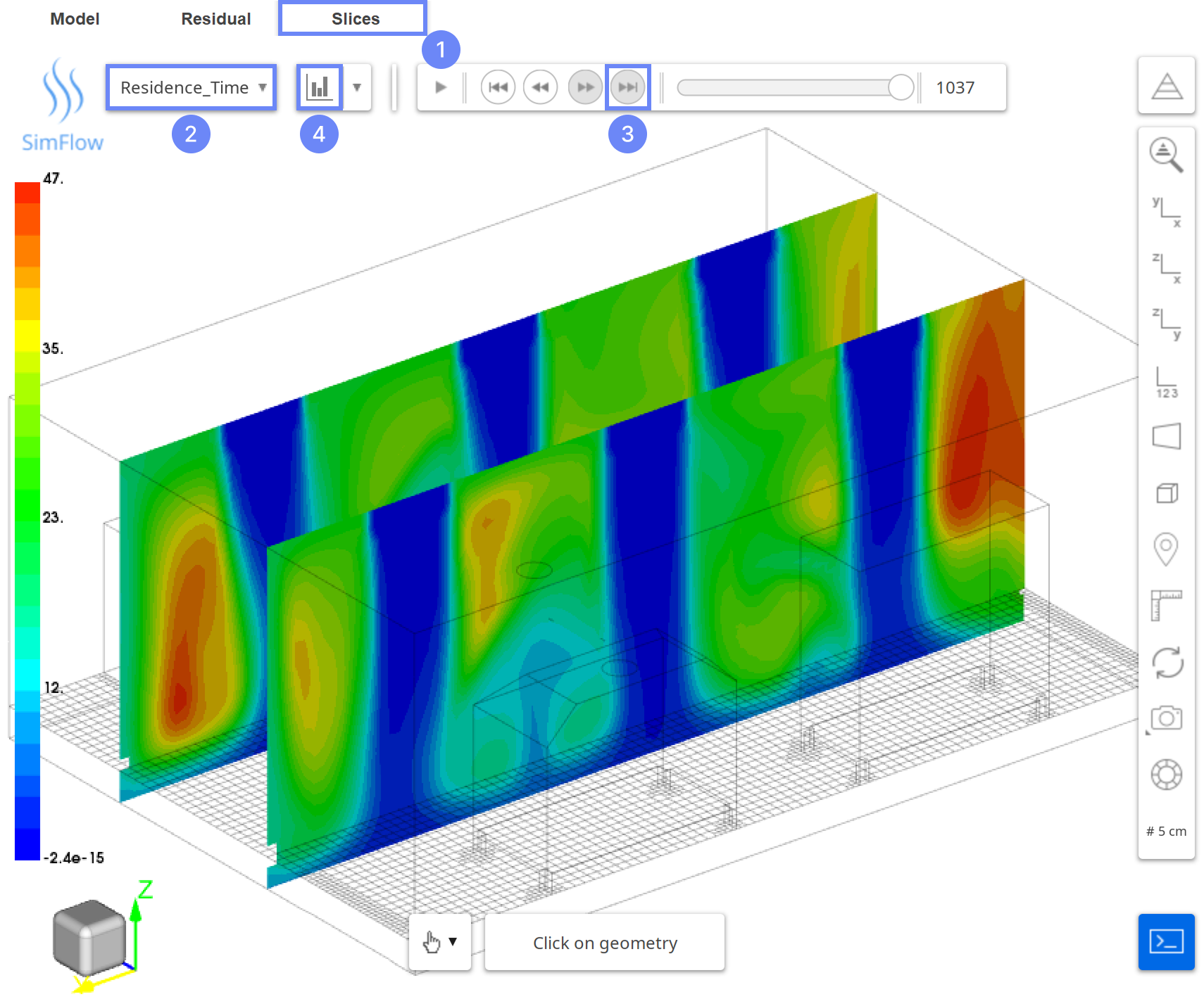
34. Slice - Residence Time
During the simulation, the Slices tab appears next to the Residuals. Under this tab, you can preview live results on the defined section planes.
- Change tab to Slices
- Select the Residence Time field
- Display results for the last iteration
- Click Adjust Range to Data
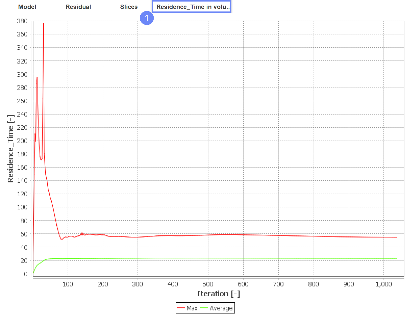
35. Residence Time Plot
Now, we can monitor the average and maximum residence time within the entire cleanroom domain during the iterations. As the calculations converge, the maximum residence time stabilizes at approximately 55 s.
- Change tab to Residence_Time in volume
36. Postprocessing - ParaView
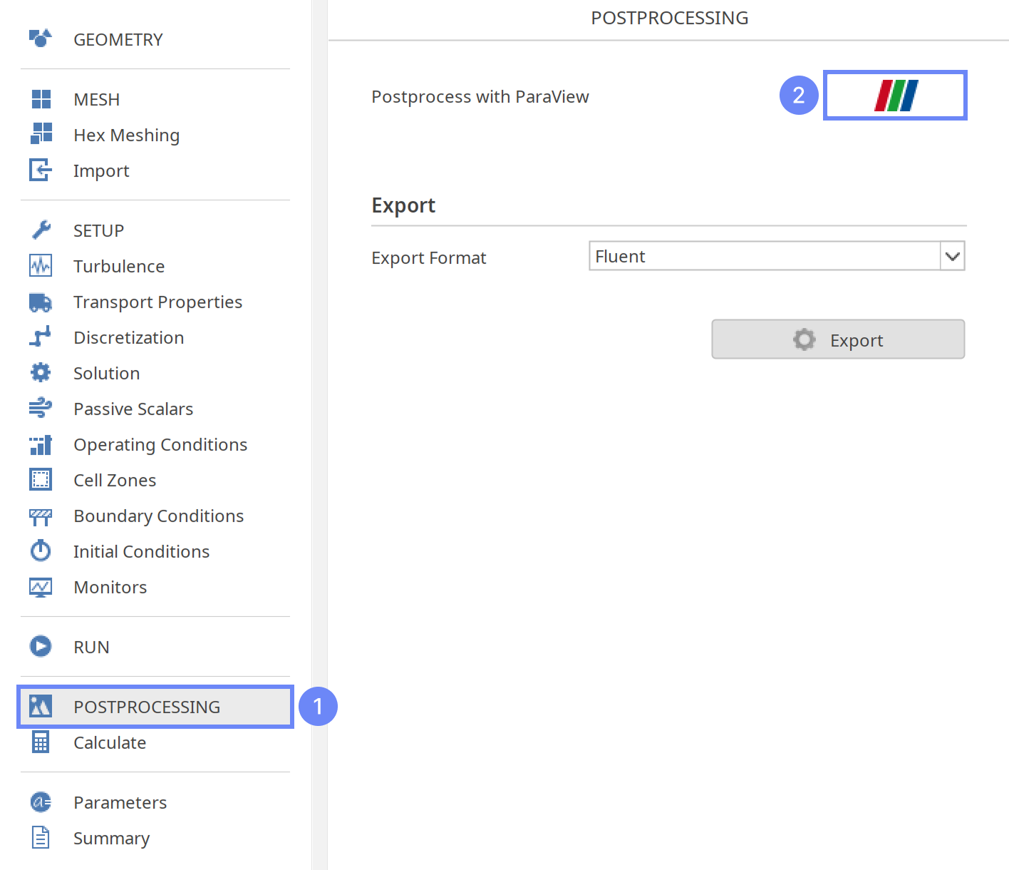
Once the computations have been completed, we can preview the stagnation region in the clean room using ParaView.
- Go to POSTPROCESSING panel
- Click on Run ParaView
37. ParaView - Load Results
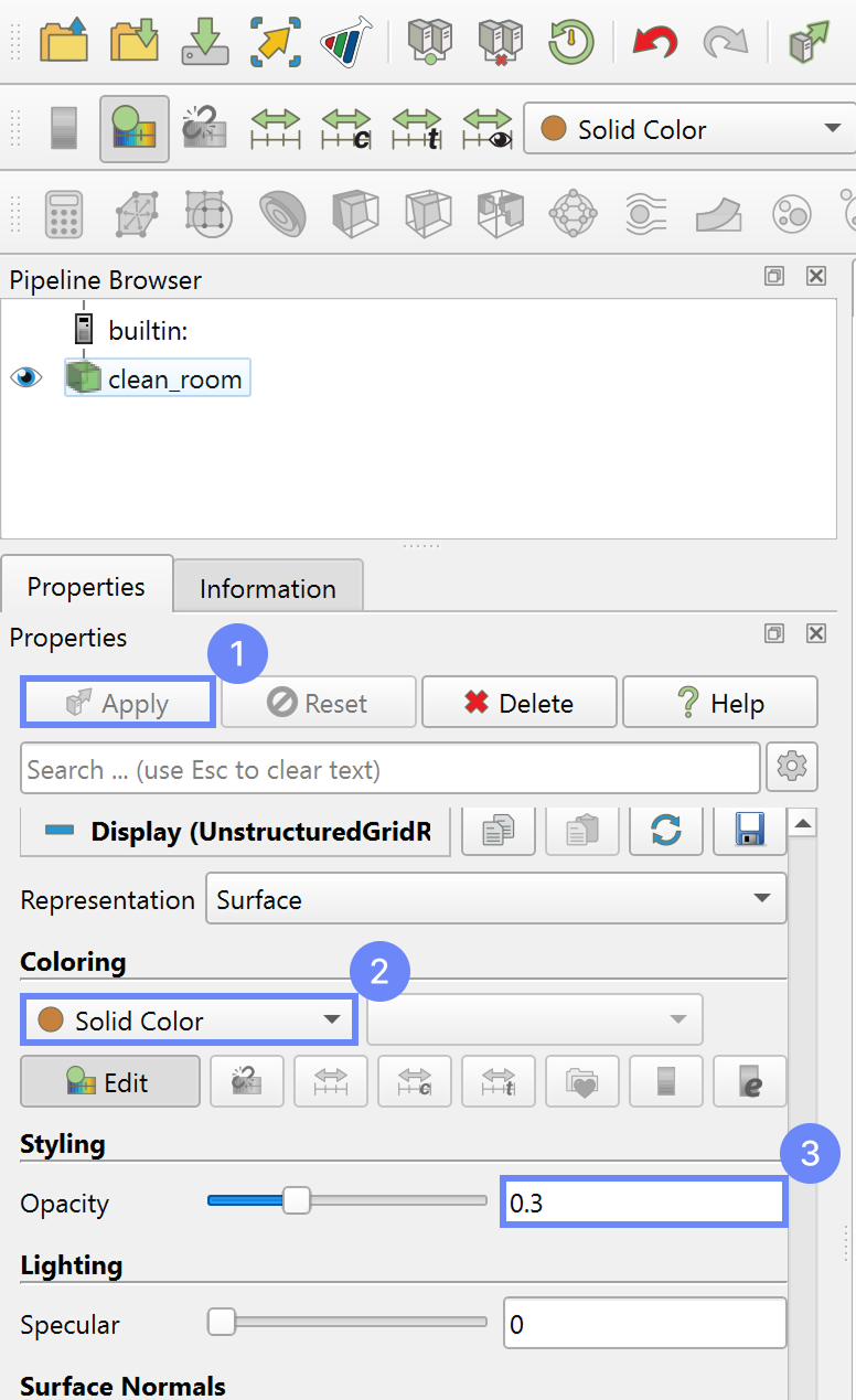
Load the results into the program.
- Click Apply to load results
- Select coloring variable to Solid Color
- Decrease the opacity
Opacity \({\sf [-]}\)0.3
38. ParaView - Create Clip
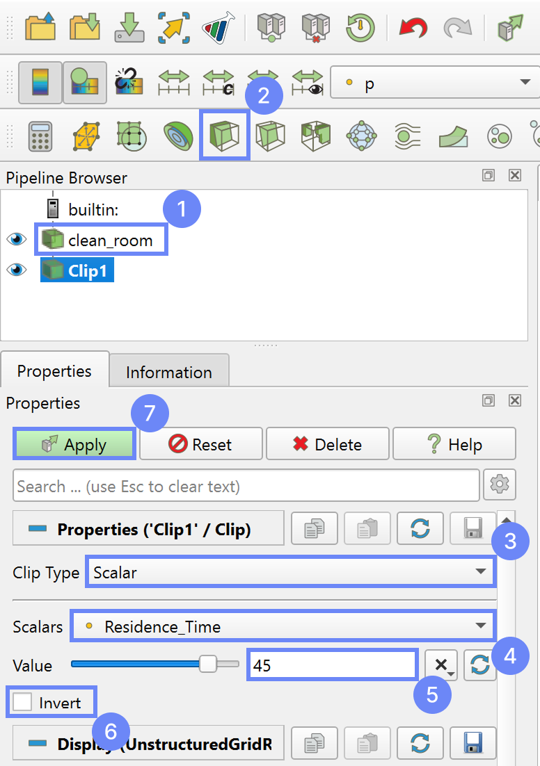
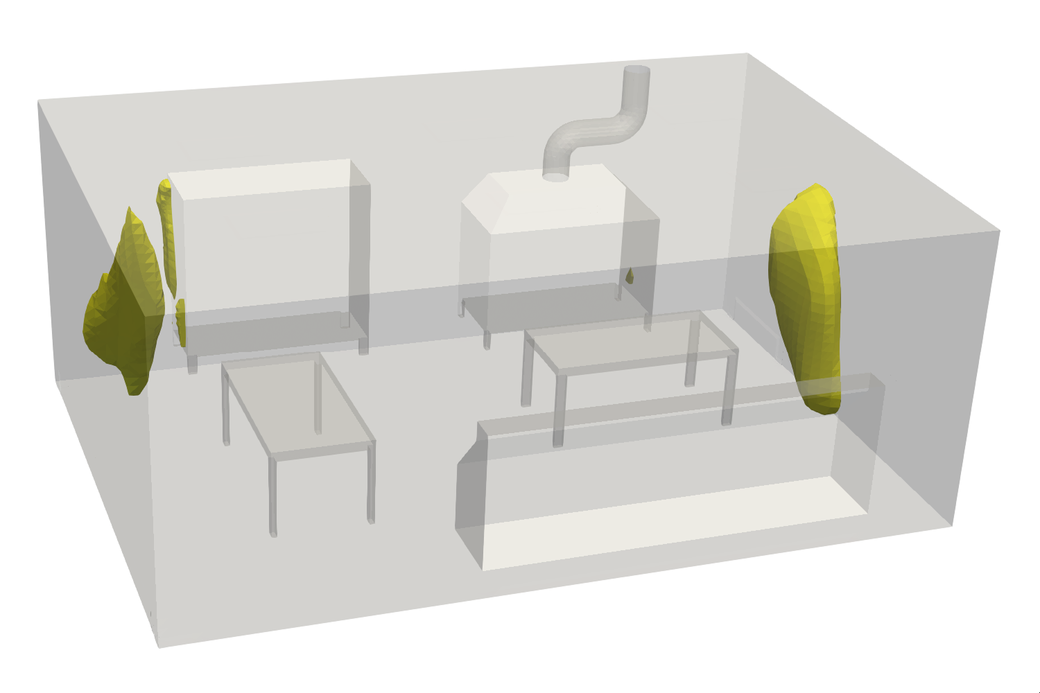
To identify regions where the air residence time exceeds a critical value, we will use the Clip filter. This filter allows us to threshold the part of the volume where a selected field variable falls outside a specified range. In this case, we will set the threshold to 45 seconds to highlight areas with higher residence time.
- Make sure your case is selected clean_room
- Create Clip
- Set Clip Type to Scalar
- Set Scalars to Residence_Time
- Define residence time threshold Value to 45
- Uncheck Invert option
- Apply changes
39. ParaView - Residence Time Results
The area can be identified as shown in the image below.
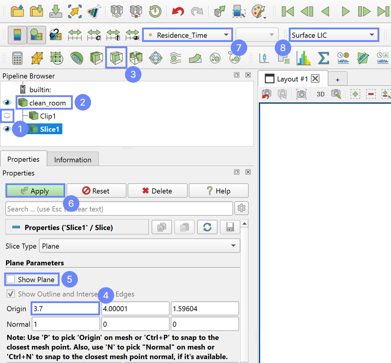
40. ParaView - Surface LIC
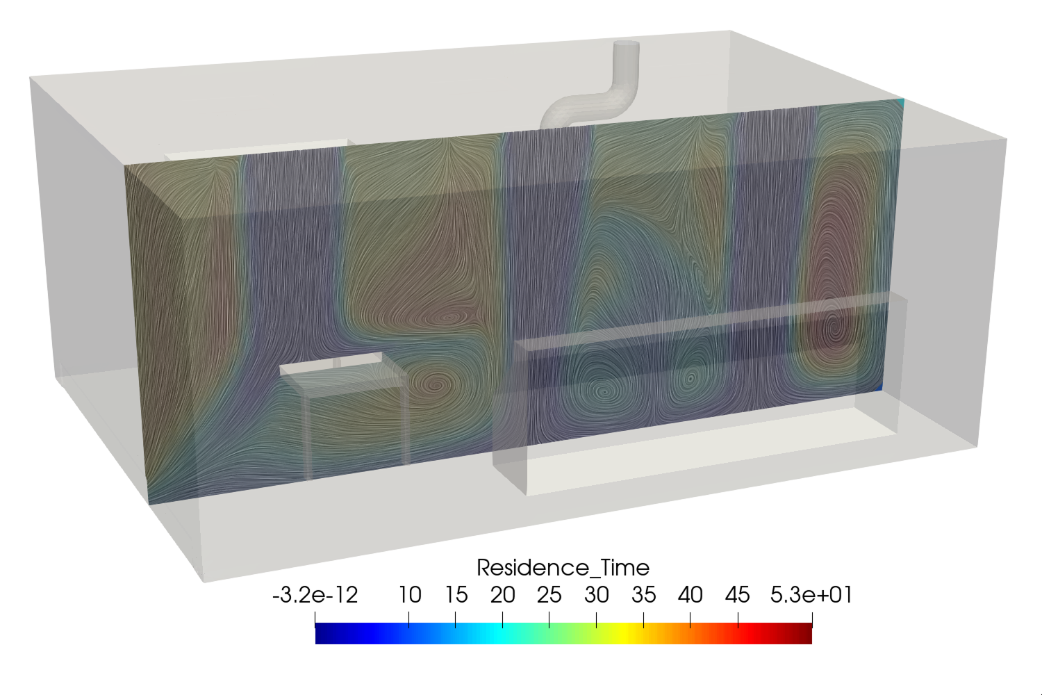
To identify the flow pattern in the region where higher residence time persists, we will visualize simplified streamlines. For this purpose, we will create a slice crossing the area of interest and display it using Surface LIC.
Surface LIC is a visualization technique that maps the flow direction and pattern directly onto a surface using texture shading. It helps reveal the flow structure without generating separate streamline objects.
- Hide the previous Clip results
- Select clean_room
- Create Slice
- Set Origin in X axis 3.7
- Uncheck Show Plane option
- Apply changes
- Select coloring variable to Residence Time
- Change the display type to Surface LIC
41. ParaView - Results
The results are shown in the image below. Areas with higher residence time are caused by flow recirculation and vortices near the inlet.