3. Create Case
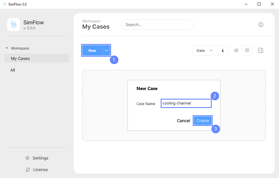
Open SimFlow and create a new case named cooling channel
- Click New
- Provide name cooling channel
- Click Create to open a new case
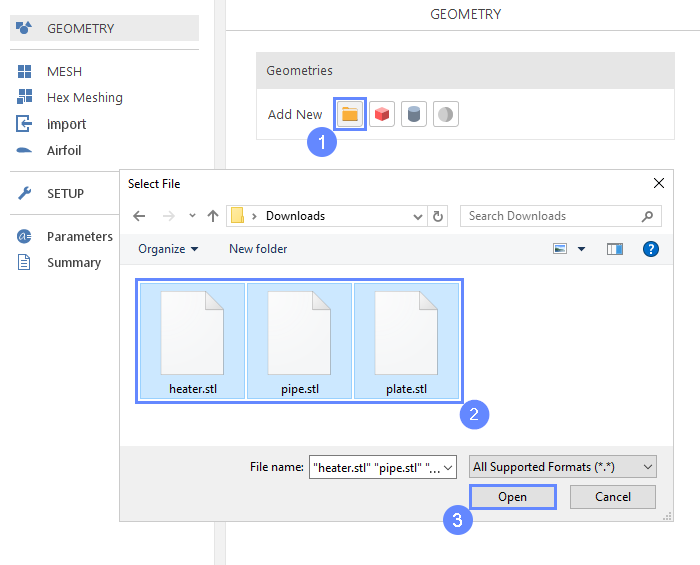
4. Import Geometry
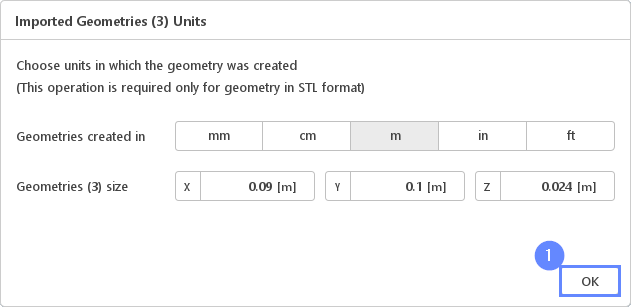
5. Imported Geometry Units
The STL format does not contain the unit information which is defined during the geometry export. If we do not know the exported unit, we can estimate it based on the total size of the model. It is displayed next to Geometry size label. In our case, the default unit meter is correct.
- Click OK button
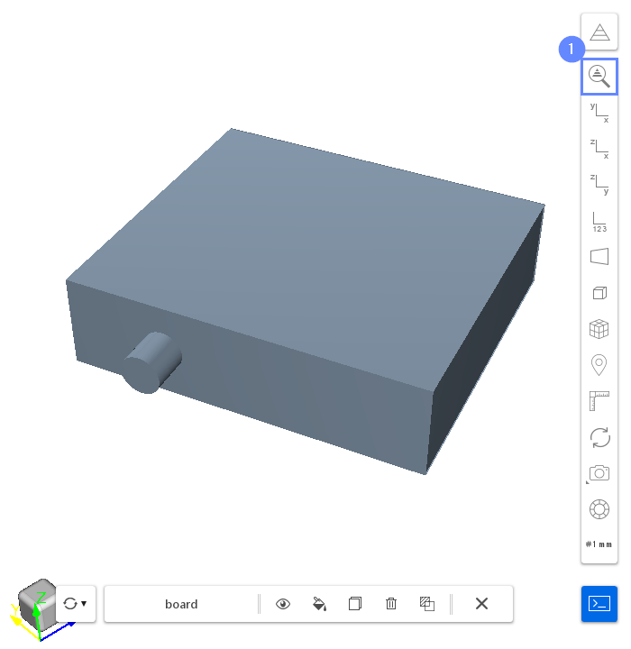
6. Geometry - Plate and Pipe
After importing geometry, it will appear in the 3D window.
- Click Fit View to fit geometry in the view
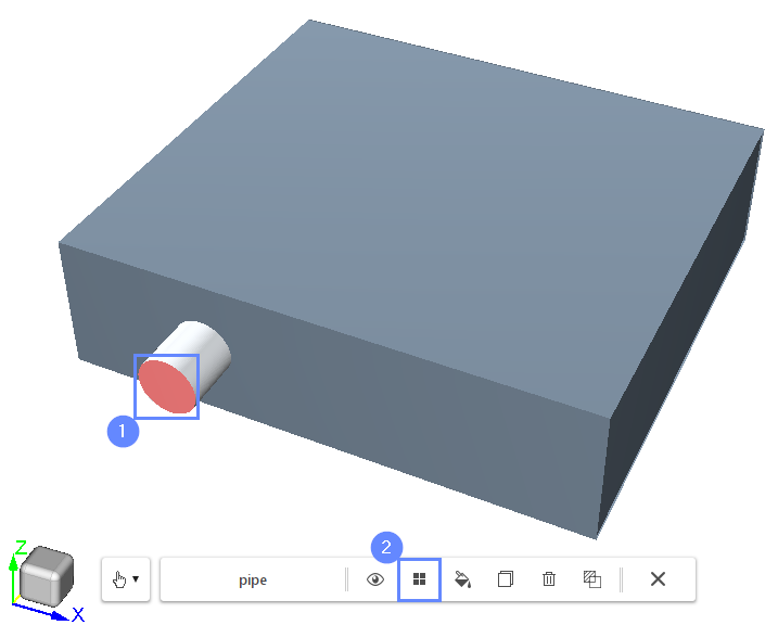
7. Creating Face Group - Inlet 1
In this simulation, we are dealing with an internal flow problem. The imported geometry determines the bounds of the domains. To inform the program where the boundaries of the inlet and outlet mesh should be created, we will use the Face Groups. Face Group is a set of faces that should be distinguished within a geometry. When the geometry containing the face group is used for meshing, an additional boundary is created. The boundary represents the respective face group and inherits its name.
- Select the inlet face by holding CTRL key and clicking on the geometry face in a 3D view. The selection should be marked in red
- Click on the Create face group from selection button in the graphics context toolbar.
New face group will be added to the current geometry - Press Esc key to clear the selection
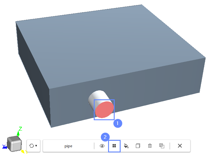
8. Creating Face Group - Outlet
Now, rotate the view in a way you will be able to see the second end of the pipe.
- Select the outlet face. Press CTRL key and click on the face
- Click on the Create face group from selection button in the context toolbar
9. Rename Face Groups
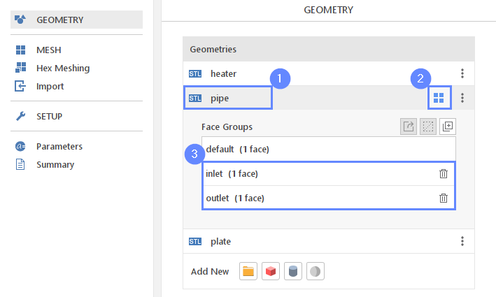
In the Geometry Panel we can find four Face Groups under the pipe geometry. The first group, named default, contains all non-selected surfaces. These surfaces will become the walls of the pipe. The two additional groups represent the inlet and the outlet of the fluid domain. We will rename these groups to make the resulting boundary names more readable.
- Select pipe geometry
- Expand Geometry Faces
- Change face groups names accordingly (double-click on a group name to start editing)
group_1 \(\rightarrow\) inlet
group_2 \(\rightarrow\) outlet
10. View Geometries I
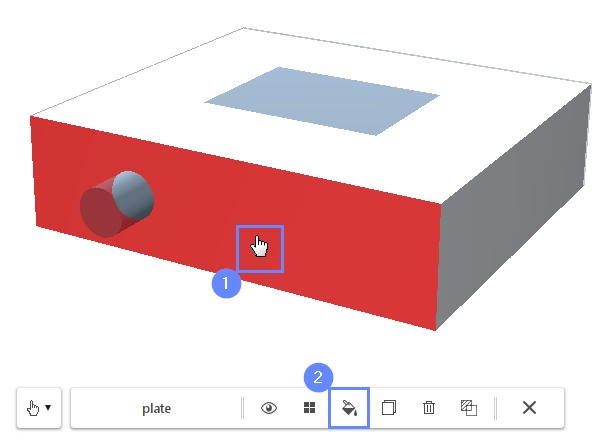
The geometry is ready to be meshed. Set the transparency of the plate geometry to see the pipe inside.
- Select plate geometry from the list or holding Ctrl key click on the plate face
- Click Change object display properties
11. View Geometries II
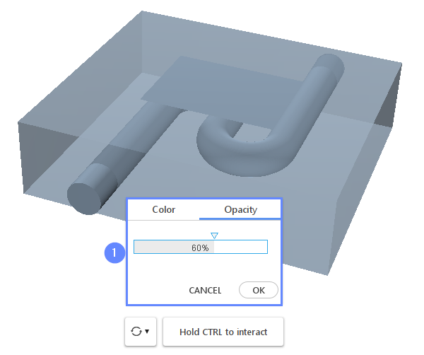
- Reduce the opacity to 60% and confirm with OK button
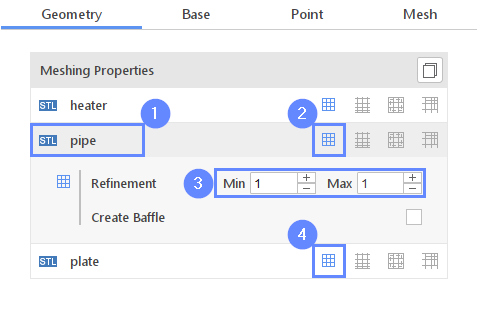
12. Meshing Properties - Heater
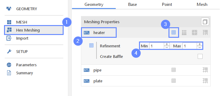
Once the geometry is prepared, we can move to the geometry surface mesh properties. To better resolve the heat transfer from the heater, we will increase mesh resolution in this area.
- Go to Hex Meshing panel
- Select heater geometry
- Enable Meshing Geometry
- Set the minimum and maximum refinement level
Refinement Min 1 Max 1
13. Meshing Properties - Pipe and Plate
Near the pipe surface, also we will refine the mesh to better resolve the coolant flow. We will apply the same settings as before.
We will also enable meshing for the plate geometry in this step.
- Select pipe geometry
- Enable Meshing Geometry
- Set the minimum and maximum refinement level
Refinement Min 1 Max 1 - Enable Meshing Geometry for the plate geometry
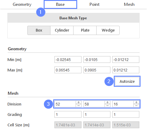
14. Base Mesh
Now, we need to define the base mesh. The box geometry determines the domain’s background mesh. The base mesh encompasses both fluid and solid regions.
- Go to Base tab
- Press Autosize button
(make sure that all geometries are visible — the Autosize adjusts the base mesh only to the visible geometry) - Define the number of divisions
Division525816
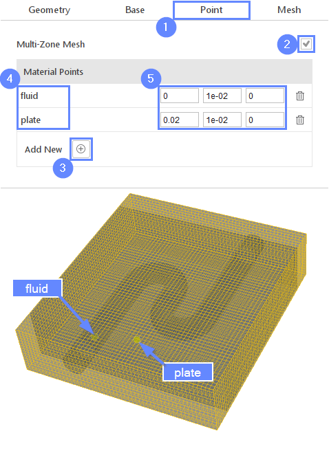
15. Material Point
Typically, we use only the default material point to create a mesh inside defined fluid volume. In this tutorial, we will take advantage of the Multi-Zone Mesh option instead. Using two material points, we will identify two separate regions in which the mesh will be created. Solid region will be used for the heat transfer in plate geometry, while in the fluid region we will simulate the fluid flow inside the pipe.
- Go to Point tab
- Check Multi_Zone Mesh option
- Add new Material Point
- Rename the material points to
fluid
plate - Set location of the material points
fluid00.010
plate0.020.010
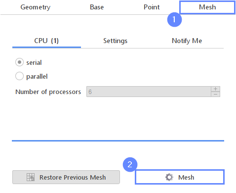
16. Meshing
In this step, we will initiate the meshing process.
The meshing process can be executed in parallel, offering a substantial reduction in mesh generation time. When running in parallel, you have the flexibility to choose the number of CPUs utilized, depending on your PC’s capabilities. Please be aware that if you are using the free version of SimFlow, you are limited to employing only 2 CPUs, and meshes exceeding 200'000 nodes cannot be created.
If you would like to test full version Request 30-day Trial
- Switch to Mesh tab
- Start the meshing process with Mesh button
17. Mesh
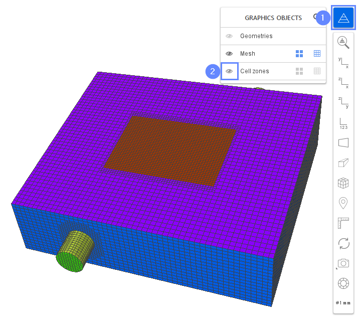
After the meshing process is finished, the mesh should appear on the screen. At the begging you will see the mesh in light blue color. All the cell zones overlap the mesh, and thus we only see the cell zones. To hide cell zones and display mesh boundaries, follow these steps:
- Expand Graphic Object List
- Click on the eye next to Cell zones
18. Create Sub-Regions
The result of multi-zone meshing is a single mesh region with multiple cell zones. At this stage, the plate and fluid volumes are connected. The boundaries separating the fluid and solid volumes are no longer present in the mesh. We can recreate them by converting the cell zones into separate mesh sub-regions. After this operation, new boundaries will appear in place where two cell zones are connected.
Please, note, when we use the Cell Zones to Regions option, the new boundaries between cell zones will be automatically coupled to each other. The coupling between boundaries localized in two different regions represents the interface that allows the heat transfer between them.
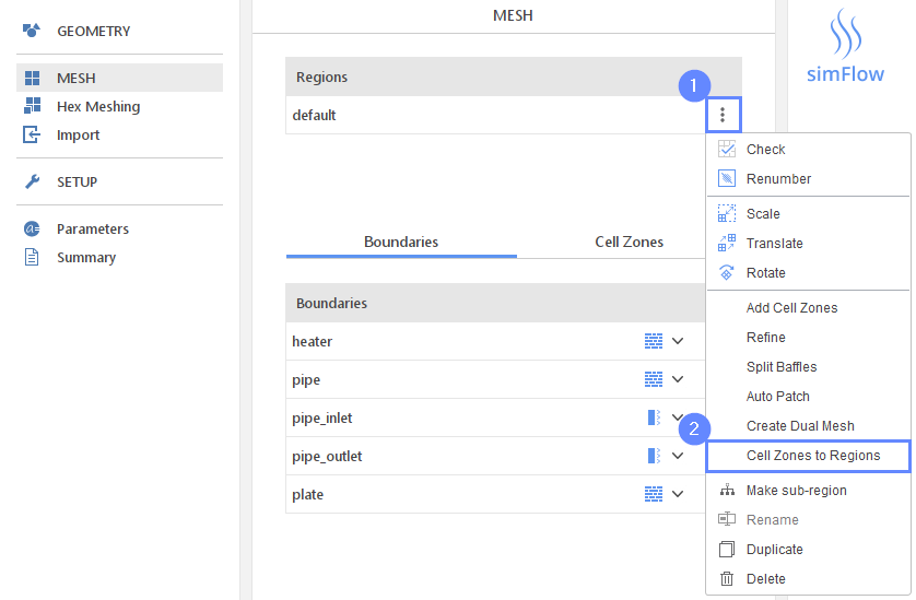
To convert cell zones to regions, you need to:
- Expand Options for the default mesh region
- Select Cell Zones to Regions option
19. Remove Default Region
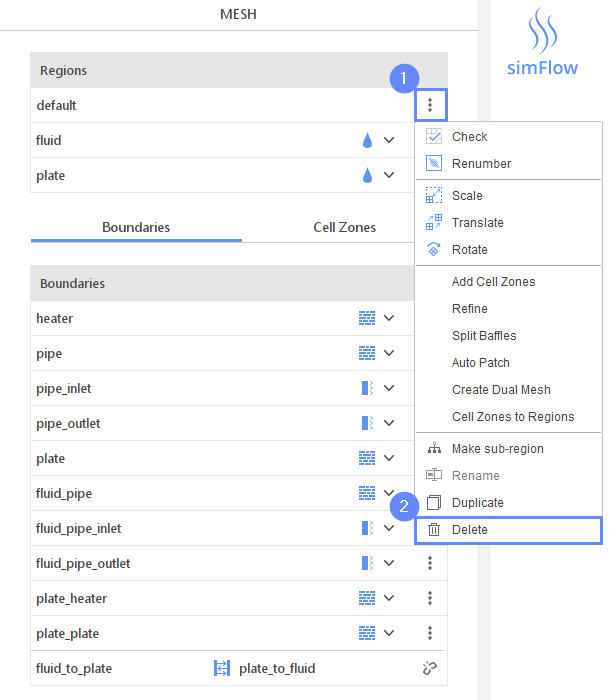
New regions appeared under the default mesh region - fluid and plate. Currently, the mesh is duplicated, and we can see both original mesh and the new regions. Now, we need to remove the old mesh (default region).
- Expand Options for the default mesh region
- Select Delete
20. Sub-Region - Solid
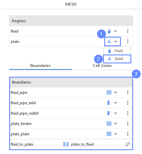
Now we will assign proper region types to indicate which region denotes fluid and solid. The default type is set as fluid which is accurate for the fluid region. However, in the case of the plate region, it is necessary to set it to solid.
Also, we need to make sure that all boundaries have the proper type. The final mesh should consist of patch types for inlet/outlet, walls for outer boundaries and the inner pipe walls interface.
- Expand the region types next to plate region
- Select Solid
- Validate boundary types to match in the image below
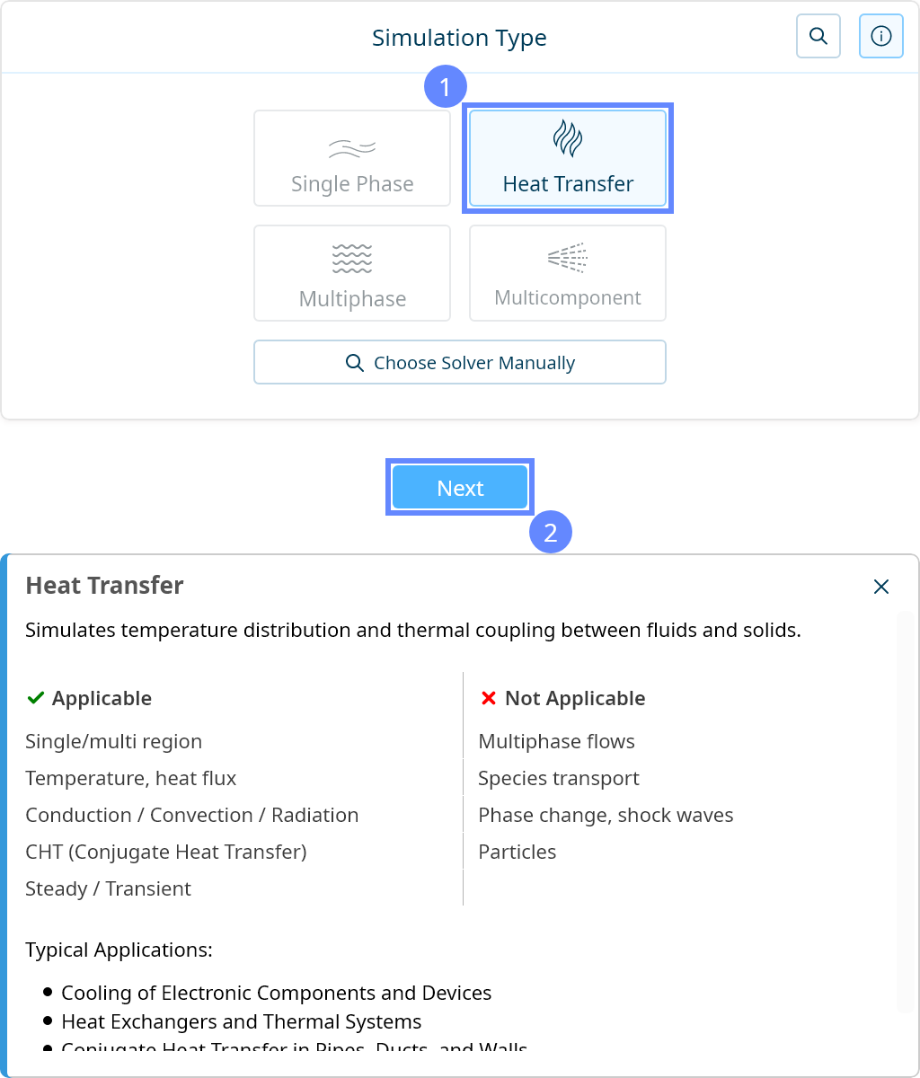
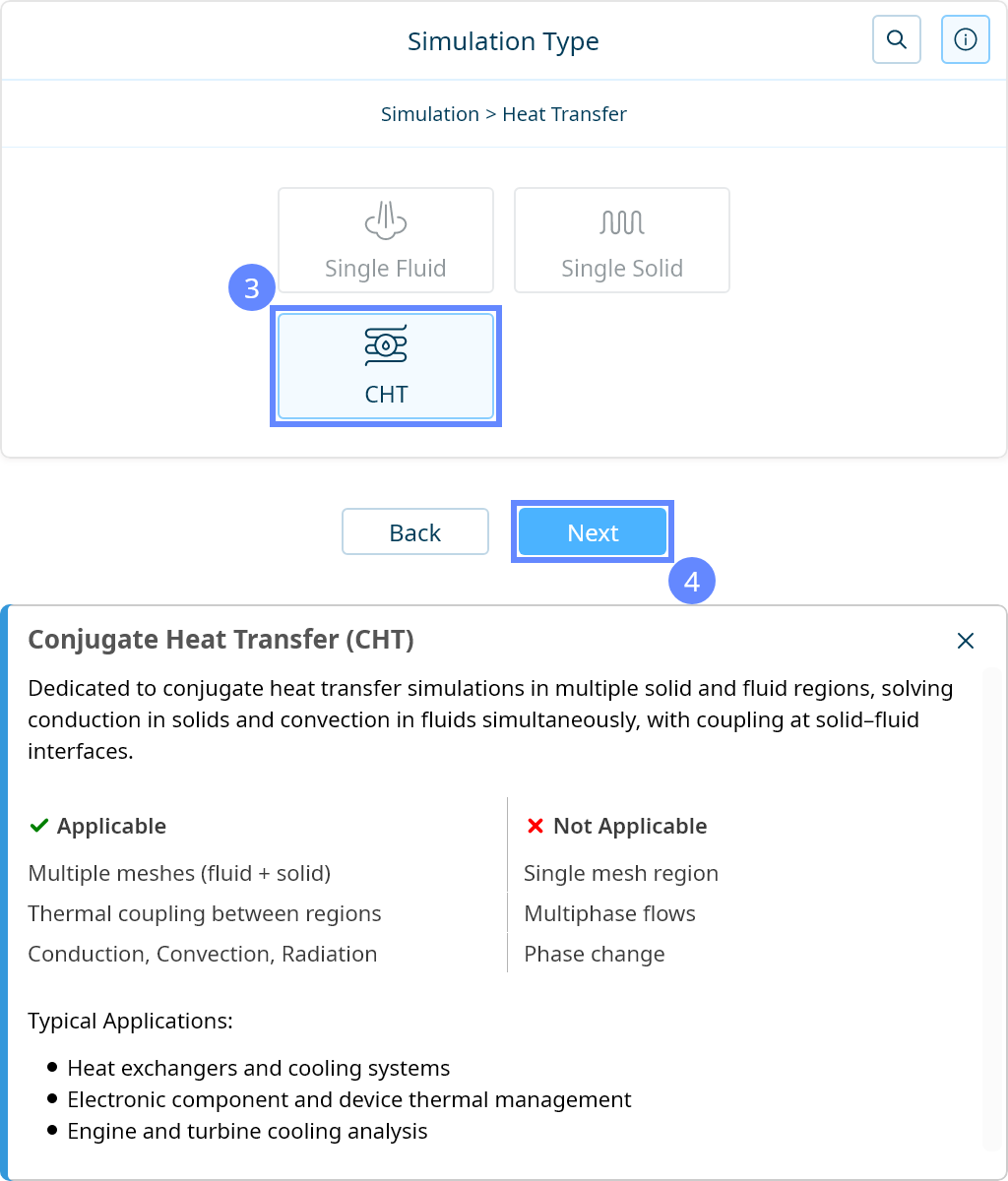
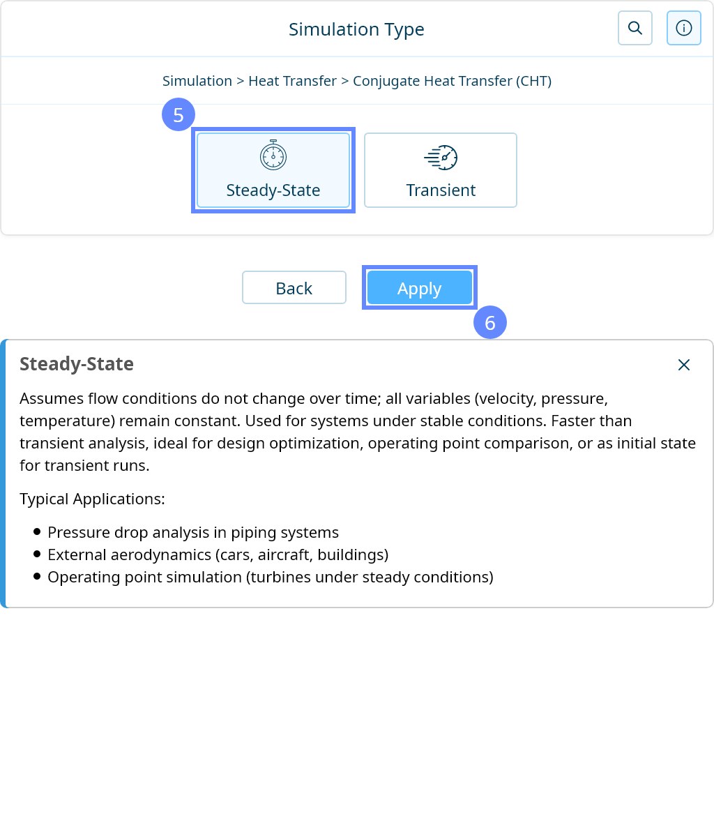
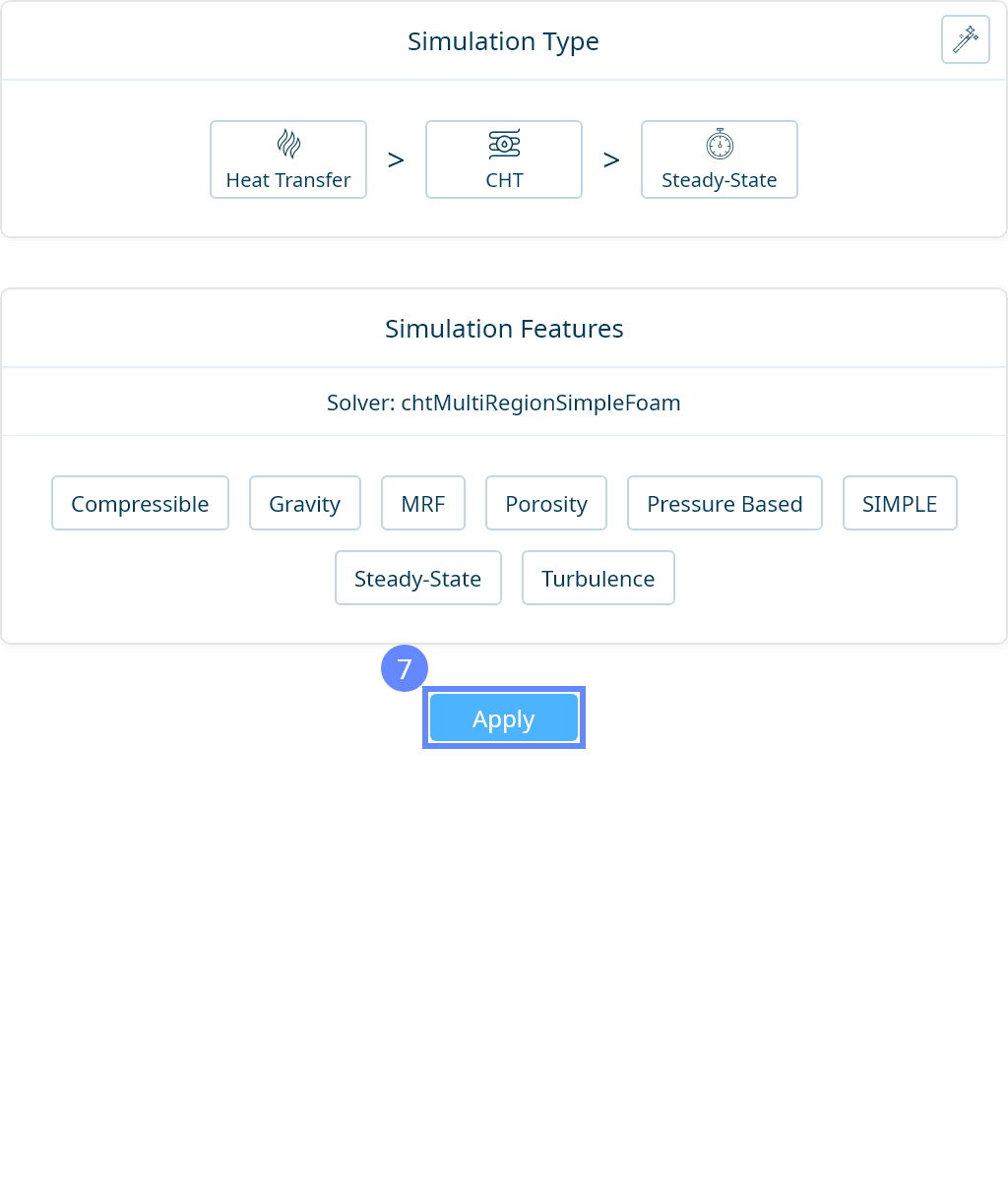
21. Simulation Type
We want to analyze the heat transfer in a cooling channel. For this purpose, we will use a steady-state conjugate heat transfer simulation.

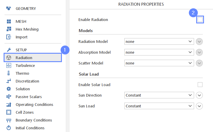
22. Radiation
For the sake of simplicity, we will not take into account the radiation heat transfer.
- Go to Radiation panel
- Uncheck Enable Radiation option
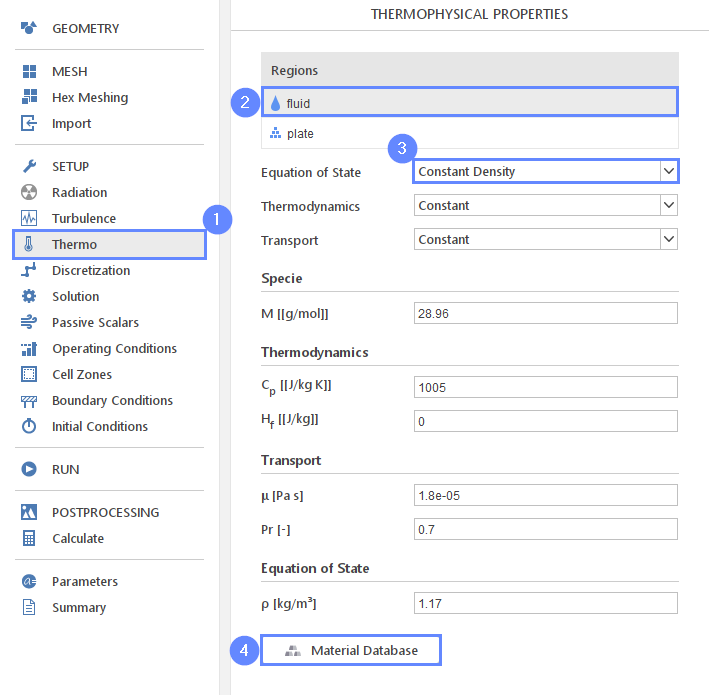
23. Thermophysical Properties - Fluid
To assign specific materials for regions, we will use the built-in database of material properties. We assume that water, incompressible fluid is flowing in the pipe.
- Go to Thermo panel
- Select fluid region
- Select Constant Density for Equation of State
- Open Material Database
Selecting material from the Material Database will fill all the inputs in the Transport Properties panel. We are still able to overwrite these values at any time.
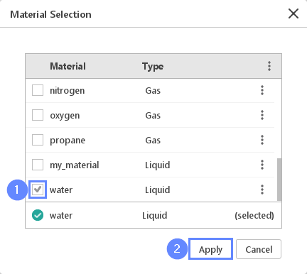
24. Thermophysical Properties - Water
- Scroll down to find water
- Click Apply
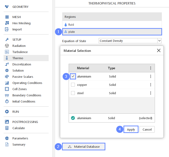
25. Thermophysical Properties - Solid
Similarly, we will now define the thermodynamic properties of a solid material. We assume that the plate is made of aluminium.
- Select solid region
- Click Material Database button
- Mark aluminium
- Click Apply
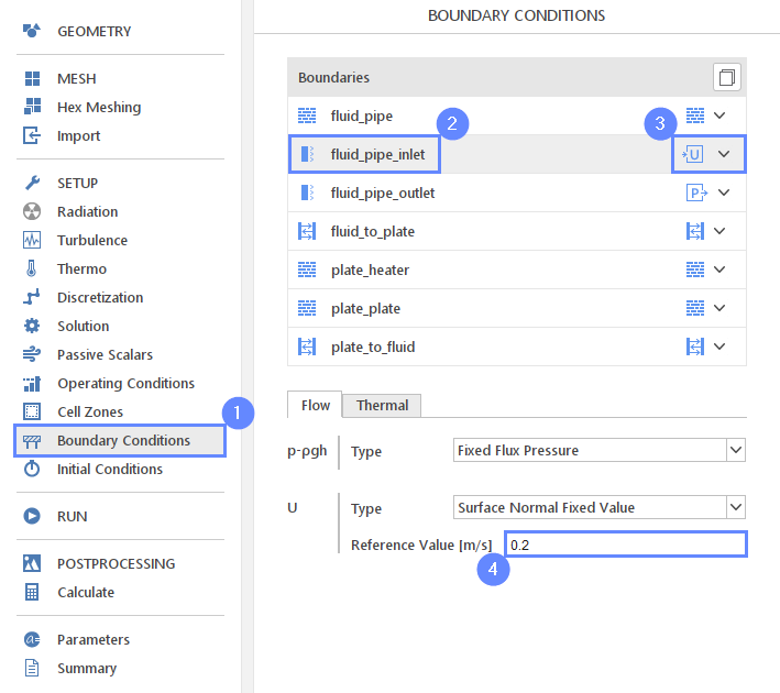
26. Boundary Conditions - Inlet (Flow)
We will now define the boundary conditions of our model. First, define the inlet velocity of the water in the pipe.
- Go to Boundary Conditions panel
- Select inlet
- Change character to velocity inlet
- Define inlet velocity
Reference Value \({\sf [m/s]}\)0.2
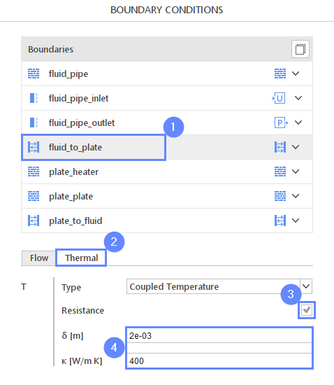
27. Thermal Boundary Conditions - Pipe
The interface between the pipe and the plate is coupled enabling the transfer of heat between these two regions. It is possible to take into account the thermal resistance of the pipe, even though the pipe thickness is not represented in the mesh. To accomplish this, you only need to specify a constant thickness of the pipe and provide its thermal conductivity.
- Select fluid_to_plate coupling interface
- Switch to Thermal tab
- Mark Resistance (if this option is not visible, select the second interface with the same name)
- Set the following parameters accordingly
\(\delta\) \({\sf [m]}\)0.002
\(\kappa\) \({\sf [W/m \cdot K]}\)400
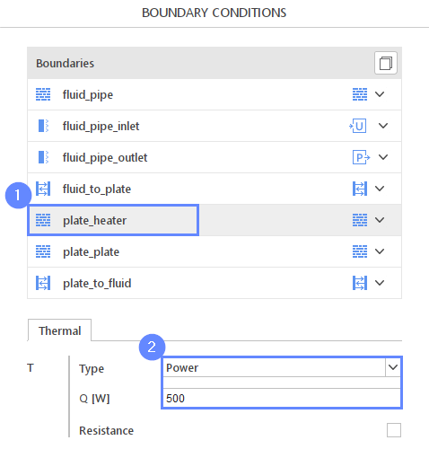
28. Boundary Conditions - Heater
To provide heat to the aluminium plate, we will use the heater boundary and assume constant heating power 'Q'.
- Select plate_heater boundary
- Set the following thermal parameters accordingly
TypePower
Q \({\sf [W]}\)500
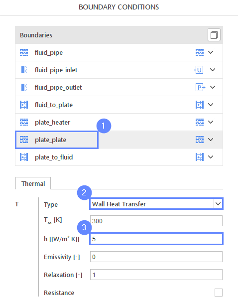
29. Boundary Conditions - Plate
To simulate the heat transfer from the plate to the environment, we will use the Wall Heat Flux boundary condition, which implements convective heat transfer. We will make the assumption that the ambient temperature is 300K, and for passive cooling, we’ll specify a heat transfer coefficient equal 5.
- Select plate_plate boundary
- 3Set the thermal parameters accordingly
TypeWall Heat Transfer
h \({\sf [W/m^2 \cdot K]}\)5
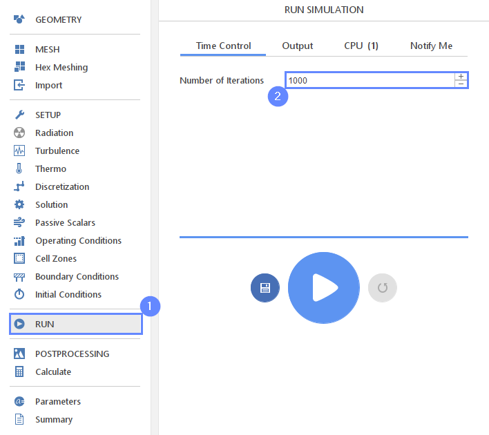
30. Run - Time Control
Finally, we can start calculations. It’s important to be aware that for the CHT solver, the maximum iteration count is the sole criterion for ending the computation. Even if the residual levels reach the desired values, the solver will continue running until the maximum iteration limit is reached.
- Go to RUN panel
- Set the maximal Numbers of Iterations to 1000
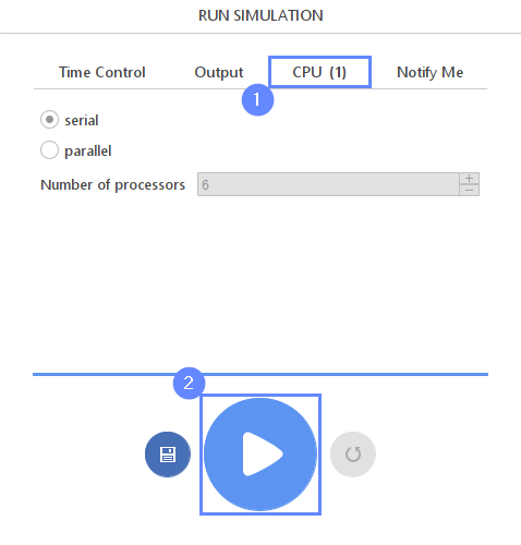
31. Run - CPU
To speed up the calculation process, take advantage of parallel computing and increase the number of CPUs based on your PC’s capability. The free version allows you to use only one processor (serial mode). To get the full version, you can use the contact form to Request 30-day Trial
Estimated computation time for serial mode: 10 minutes
- Switch to CPU tab
- Click Run Simulation button
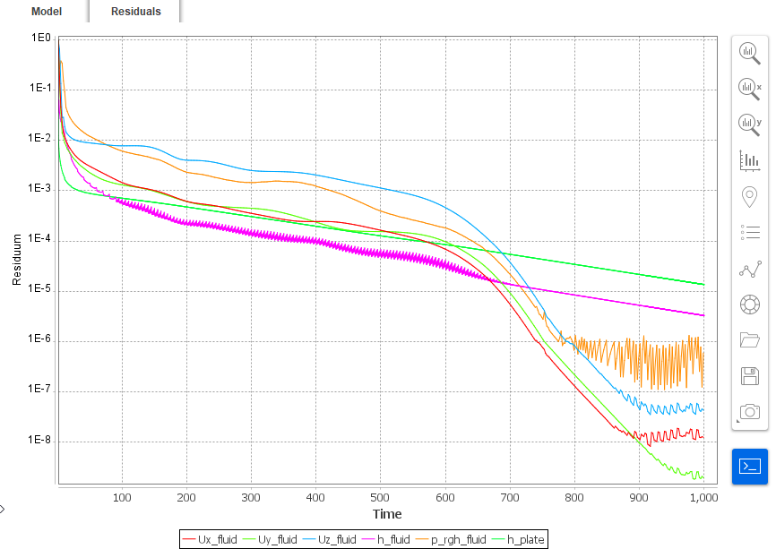
32. Residuals
When the calculation is finished, we should see a similar residual plot.
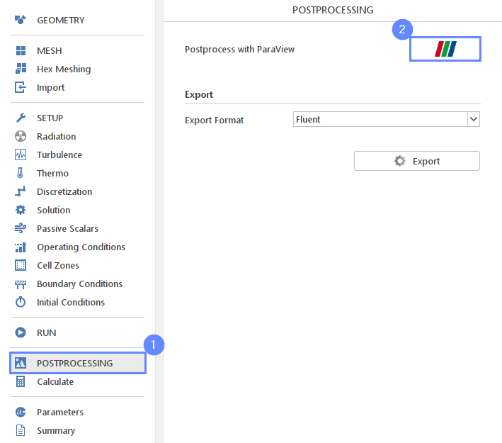
33. Start Postprocessing with ParaView
Start ParaView software to display results.
- Go to Postprocessing panel
- Run ParaView
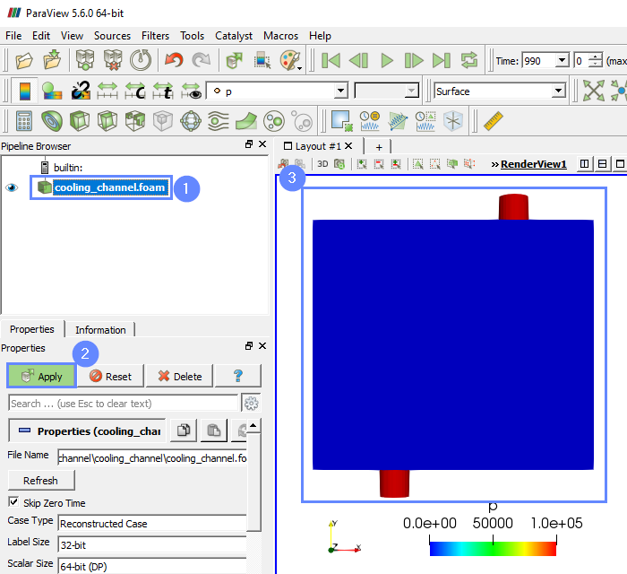
34. ParaView - Load Results
Load results into the ParaView.
- Select cooling_channel.foam
- Click Apply to load results into ParaView
- After loading results, they will be shown in the 3D graphic window
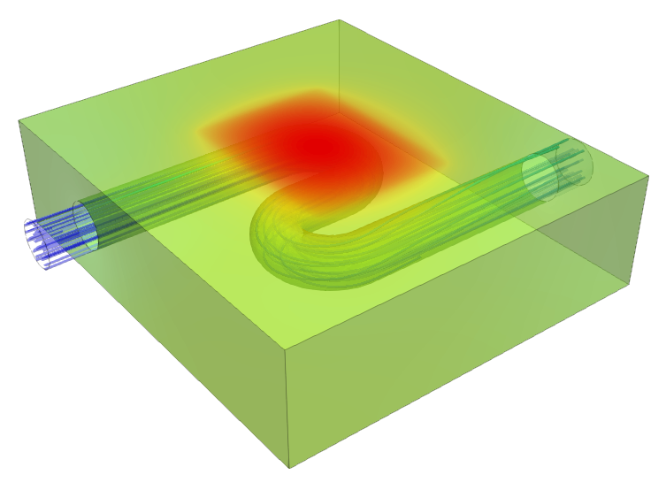
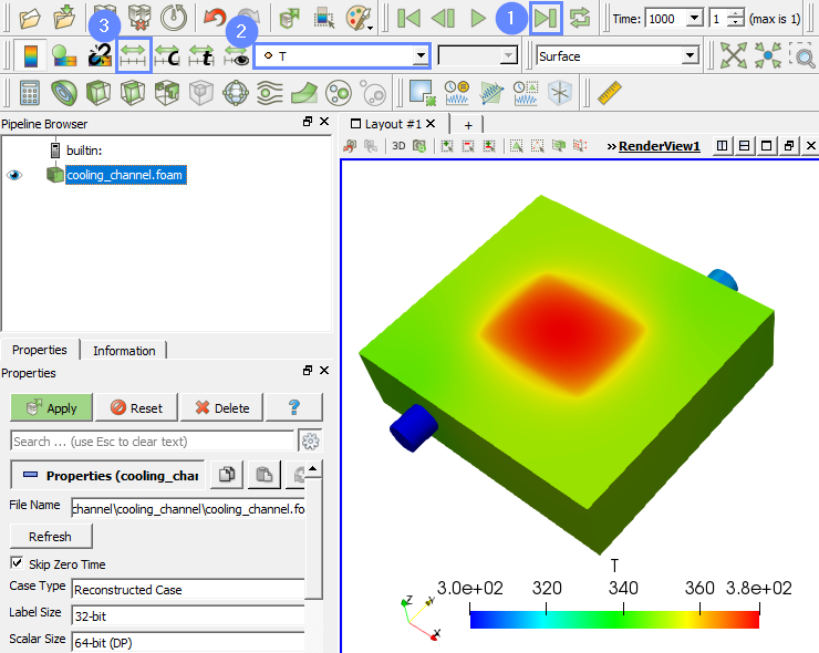
35. ParaView - Display Temperature Contour (I)
We will display the temperature map for the model.
- Click Last Frame
- Select contour coloring variable to T
- Click Rescale to Data Range
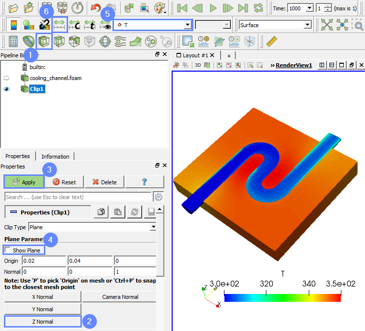
36. ParaView - Display Temperature Contour (II)
To see the temperature distribution inside the model, we will use the clip filter.
- Select Clip
- Set the clip plane along Z Normal
- Click Apply
- To hide plane uncheck option Show Plane
- Select contour coloring variable to T
- Click Rescale to Data Range