3. Create Case
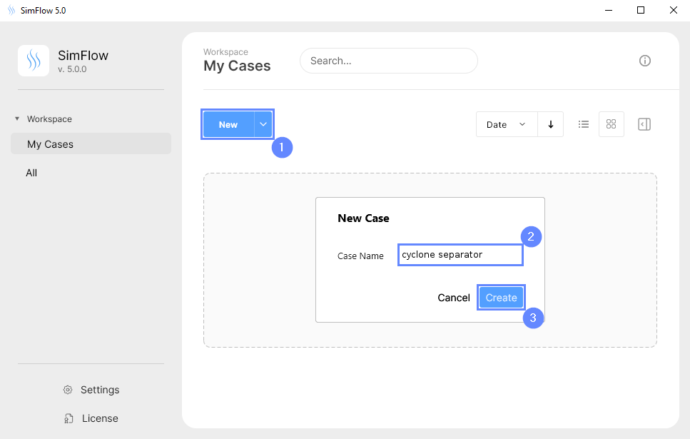
Open SimFlow and create a new case named cyclone separator
- Click New
- Provide name cyclone separator
- Click Create to open a new case
4. Import Geometry
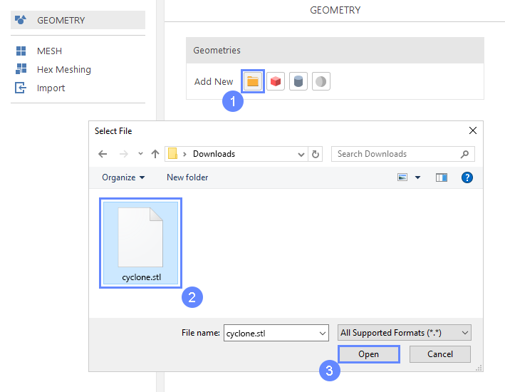
After creating case Download GeometryCyclone
- Click Import Geometry
- Select geometry file cyclone.stl
- Click Open
5. Imported Geometry Units
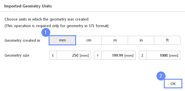
The STL format does not contain the unit information which are defined during the geometry export. Therefore, you must manually specify the correct unit after import. If we do not know the exported unit, we can estimate it based on the total size of the model. It is displayed next to Geometry size label. In our case, the model was created in millimeters.
- Select mm unit
- Click OK button
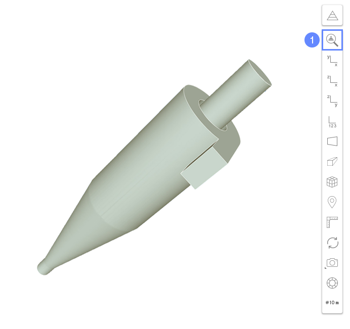
6. Display Geometry
After importing geometry, it will appear in the 3D window
- Click Fit View to zoom out the geometry
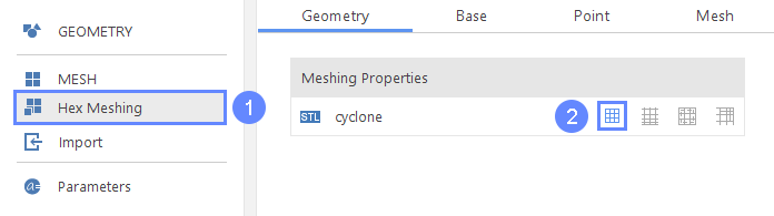
7. Meshing Parameters - Cyclone
Now we will set meshing parameters for cyclone geometry
- Go to Hex Meshing panel
- Enable meshing on the cyclone geometry
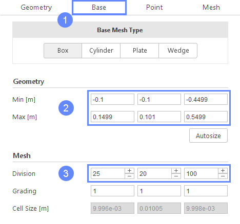
8. Base Mesh
We will define the base mesh now
- Go to Base tab
- Define initial mesh extends
Min \({\sf [m]}\)-0.1-0.1-0.4499
Max \({\sf [m]}\)0.14990.1010.5499
(these dimensions have been set, so that inlet, bottom and top faces of the geometry fall slightly outside the box) - Define the number of divisions
Division2520100
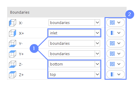
9. Base Mesh Boundaries
To create separate boundaries at the intersections of the base mesh with the geometry, we need to assign them individual names and types.
- Change the following boundary names accordingly
X+ inlet
Z- bottom
Z+ top - Define boundary types accordingly
X- wall
X+ patch
Y- wall
Y+ wall
Z- wall
Z+ patch
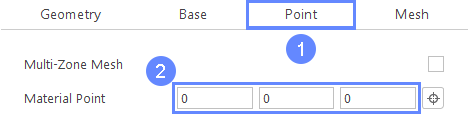
10. Material Point
Make sure the material point is located inside the geometry
- Go to Point tab
- Make sure that the material point is set accordingly
Material Point000
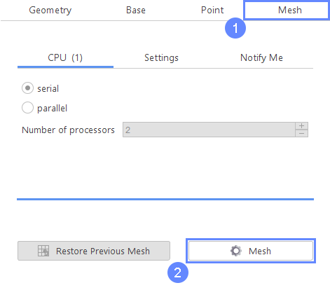
11. Start Meshing
Now everything is set up, we can begin the meshing process
- Go to Mesh tab
- Click Mesh to start the meshing process
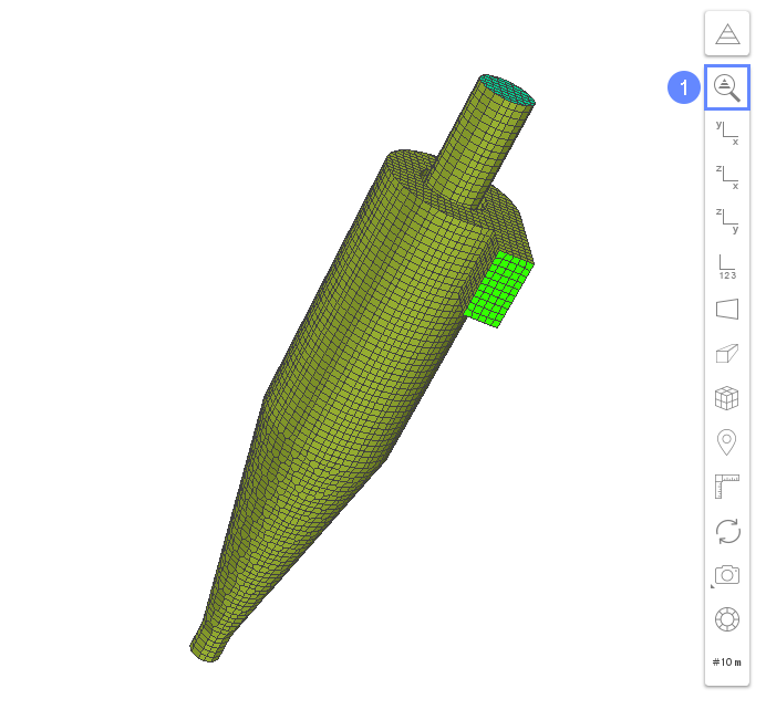
12. Mesh
After meshing process is finished the mesh should appear in the 3D graphics window
- Click Fit View
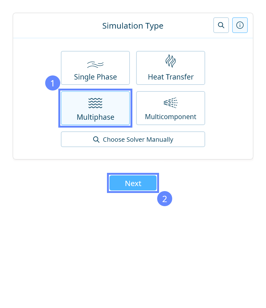
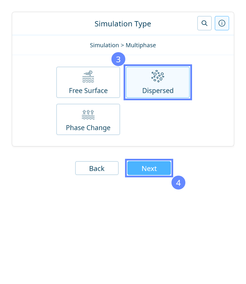
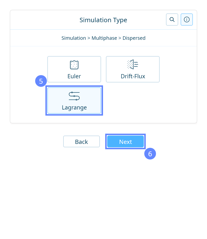
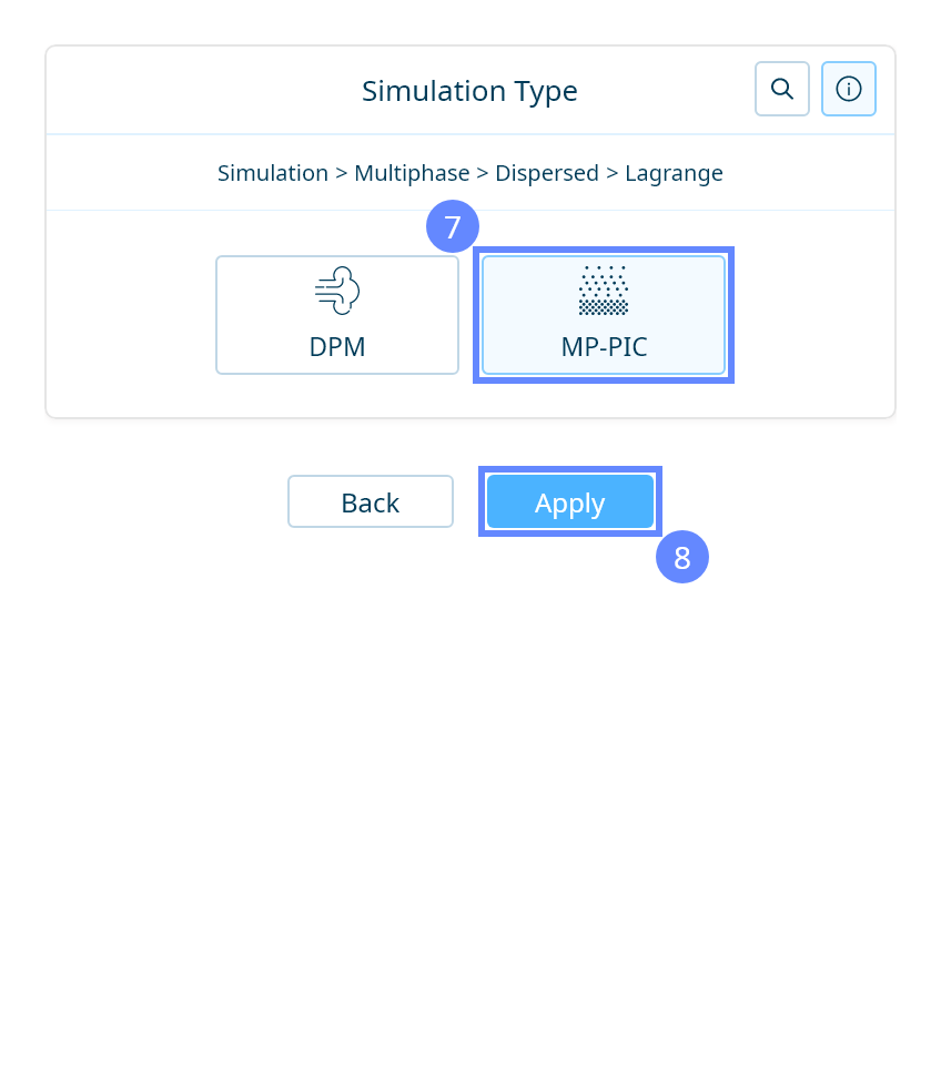
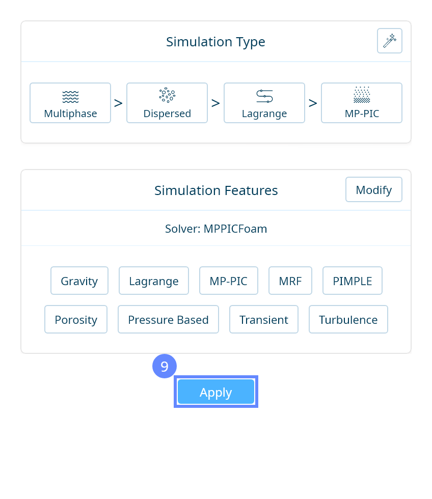
13. Simulation Type
We want to analyze the particle separation in a cyclone. For this purpose, we will use a multiphase transient simulation of fluid flow with Lagrangian particles using the MP-PIC method.

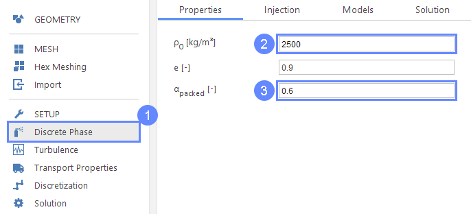
14. Discrete Phase - Properties
We will now define properties of the discrete phase
- Go to Discrete Phase panel
- Set density of the discrete phase
\(\rho_0\) \({\sf [\frac{kg}{m^2}]}\)2500 - Set packing factor
\(\alpha_{packed}\) \({\sf [-]}\)0.6
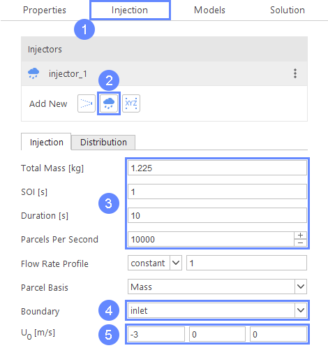
15. Discrete Phase - Injection
We will now define the injection of the discrete phase through the inlet boundary.
- Go to Injection tab
- Create Boundary Injector
- 45 Set following parameters accordingly
Total Mass \({\sf [kg]}\)1.225
SOI \({\sf [s]}\)1
Duration \({\sf [s]}\)10
Parcels Per Second10000
Boundaryinlet
\(U_0\) \({\sf [m/s]}\)-300
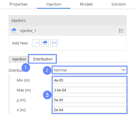
16. Discrete Phase - Distribution
We will now define a normal distribution of the discrete phase size
- Go to Distribution tab
- Set Distribution to Normal
- Set distribution parameters accordingly
Min \({\sf [m]}\)4e-05
Max \({\sf [m]}\)3.6e-04
\(\mu\) \({\sf [m]}\)5e-05
\(\sigma\) \({\sf [m]}\)2e-04
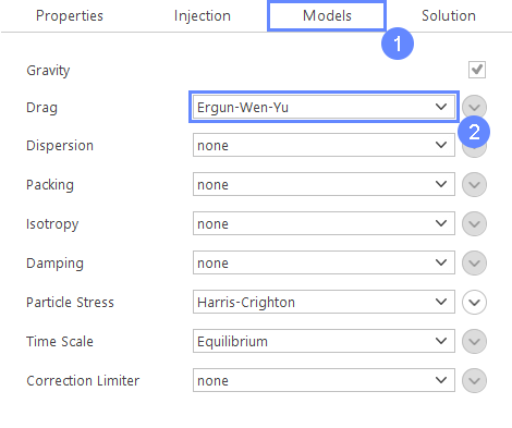
17. Discrete Phase - Models
We will now define the particle drag model
- Go to Models tab
- Select Ergun-Wen-Yu model
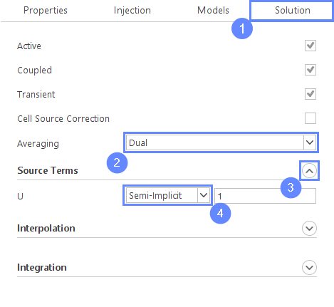
18. Discrete Phase - Solution
We will now define methods of computing and interpolating an average of the Lagrangian phase
- Go to Solution tab
- Set Averaging method to Dual
- Expand Source Terms options
- Set Semi-Implicit discretization of the U term
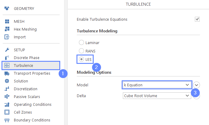
19. Turbulence
For turbulence modeling, we will use the LES model
- Go to Turbulence panel
- Select LES turbulence modeling
- Select \(k \; Equation\) model
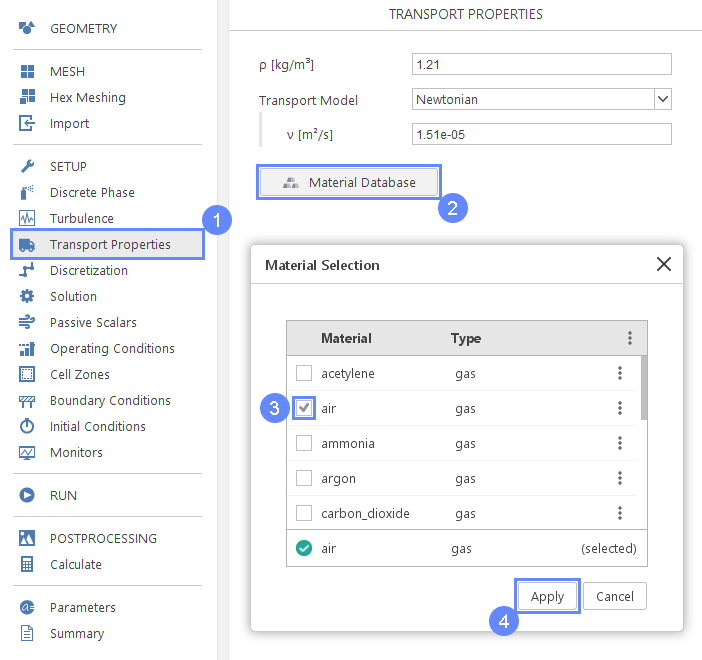
20. Transport Properties - Fluid
Now we will define the transport properties of fluid material
- Go to Transport Properties panel
- Click Material Database
- Select air material
- Click Apply
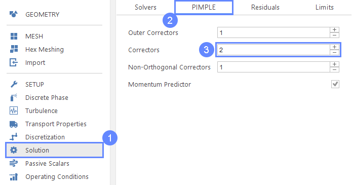
21. Solution - PIMPLE
To increase the stability of the simulation we will increase the number of pressure corrector iterations
- Go to Solution panel
- Select the PIMPLE tab
- Increase the number of Correctors to 2
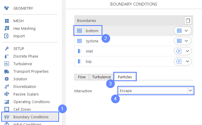
22. Boundary Conditions - Bottom (Particles)
Now we will set how particles interact with boundaries. The Bottom boundary should be transmissive for particles.
- Go to Boundary Conditions panel
- Select bottom boundary
- Select Particles tab
- Change particle interaction to Escape
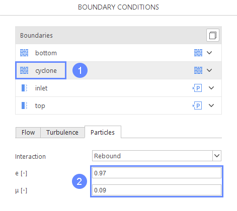
23. Boundary Conditions - Cyclone (Particles)
- Select cyclone boundary
- Set following values accordingly
e \({\sf [-]}\)0.97
\(\mu\) \({\sf [-]}\)0.09
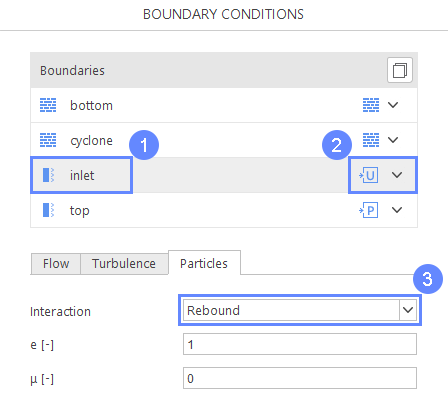
24. Boundary Conditions - Inlet (Particles)
We will now set boundary conditions on inlet boundary
- Select inlet boundary
- Change boundary condition for inlet to Velocity Inlet
- Change particle interaction to Rebound
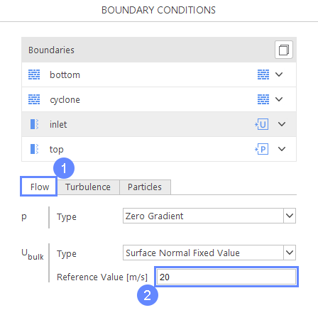
25. Boundary Conditions - Inlet (Flow)
- Switch to Flow tab
- Set velocity at inlet
Reference Value \({\sf [m/s]}\)20
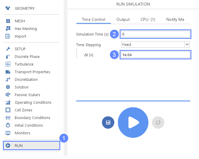
26. Run - Time Controls
Finally, we can start our computation.
- Go to Run panel
- Set Simulation Time [s] to 5
- Set time step \(\Delta t [s]\) to 1e-04
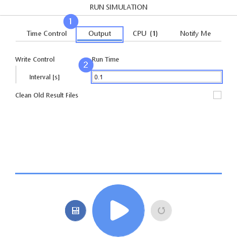
27. Run - Output
- Go to Output tab
- Set Write Control Interval [s] to 0.1 seconds
(it will force solver to write results on the hard drive every 0.1 seconds of the simulation)
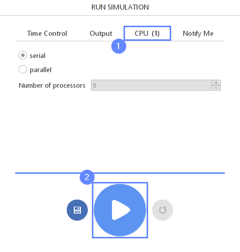
28. Run - CPU
To speed up the calculation process, take advantage of parallel computing and increase the number of CPUs based on your PC’s capability. The free version allows you to use only one processor (serial mode). To get the full version, you can use the contact form to Request 30-day Trial
Estimated computation time for serial mode: 6 hours
- Switch to CPU tab
- Click Run Simulation button
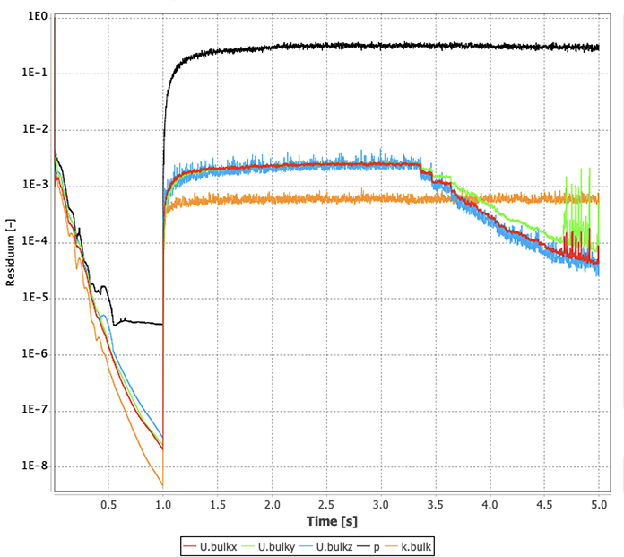
29. Residuals
When the calculation is finished, we should see a similar residual plot.
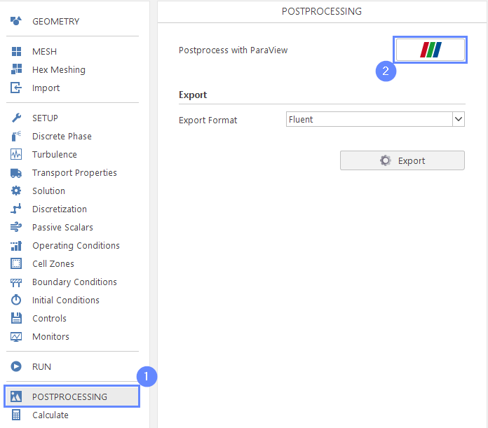
30. Postprocessing - Open ParaView
Open ParaView software to display results
- Go to Postprocessing panel
- Start ParaView
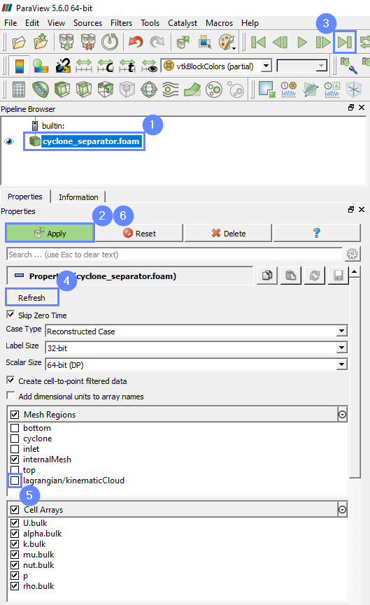
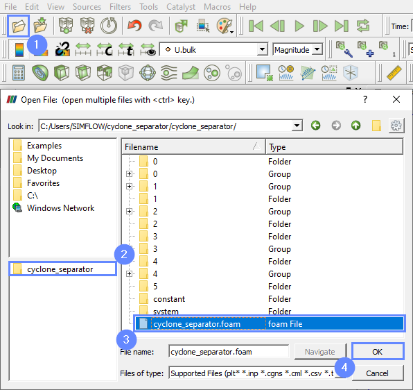
31. ParaView - Import Results
After opening the ParaView we will import result from the simulation. We will import fluid region and parcels cloud separately to be able to assign them different display properties.
- Select cyclone_separator.foam
- Click Apply to import results
- Click Last Frame to select the latest result set
- Refresh the results
- Uncheck lagrangian/kinematicCloud region
- Click Apply
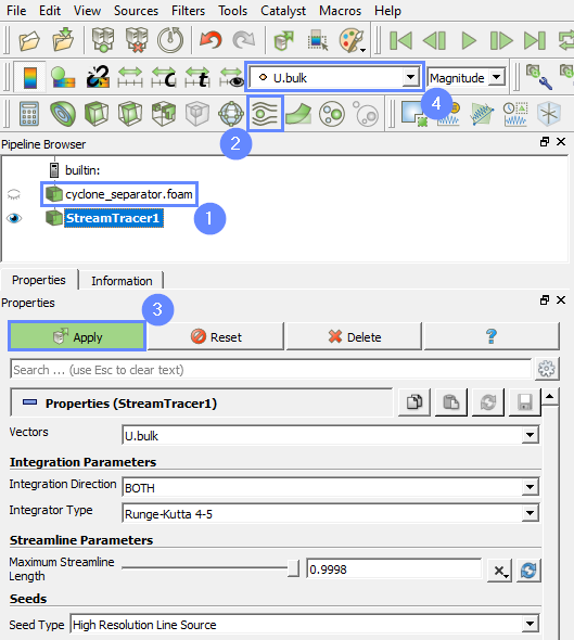
32. ParaView - Streamlines
We will now plot streamlines for the fluid region and set the coloring variable to velocity
- Select cyclone_separator.foam
- Click Stream Tracer button to add streamlines
- Click Apply
- Change the coloring variable to U.bulk
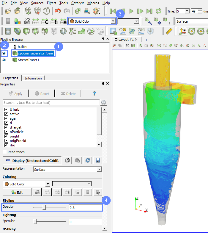
33. ParaView - Display Geometry
To show the transparent geometry together with the streamlines we will follow below steps:
- Select cyclone_separator_foam
- Click on the eye next to cyclone_separator_foam
- Select Solid Color from the list
- Change the opacity in a properties tab to 0.3
34. ParaView - Display Particles (I)
In order to display particles you can import the same case into ParaView once again
- Select Open from the top menu
- Make sure you are in folder with cyclone_separator_foam case
- Select cyclone_separator.foam from file
- Click OK
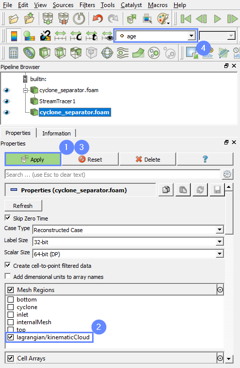
35. ParaView - Display Particles (II)
Now we will select to display particles only
- Click Apply
- Go to Mesh regions, uncheck all regions and check only lagrangian/kinematicCloud
- Click once again Apply to confirm
- Change the coloring variable to the age
| Note that after first applying, lagrangian/kinematicCloud will appear on the list of mesh regions. |
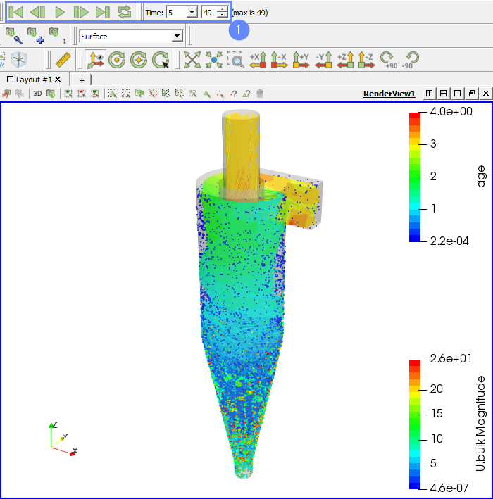
36. ParaView - Results
The results are displayed in the graphics window.
- Play with an animation buttons to track the results of analysis
| Note that this tutorial is meant only to demonstrate the capabilities of the software and not to solve the problem in the best possible way. Therefore, some assumptions are taken to keep case setup time and computational time low. In particular, to refine the model, one could in the first place consider refining the mesh and choosing a more suitable drag model for the particles (e.g. Ergun-Wen-Yu model). Subsequently, it is worth considering enabling isotropic particle packing, isotropic particle timescale, and stochastic isotropy model. |