3. Create Case
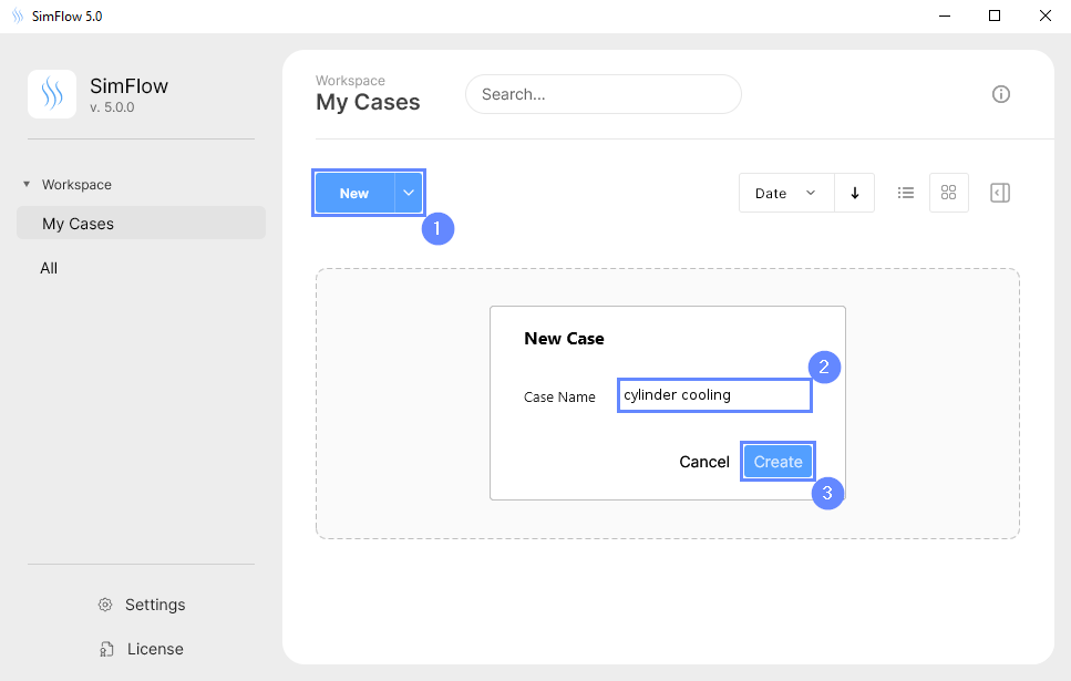
Open SimFlow and create a new case named cylinder cooling
- Click New
- Provide name cylinder cooling
- Click Create to open a new case
4. Create Geometry - Cylinder
We need to create a cylindrical boundary for the domain. For this purpose, we will create a cylindrical geometry for later use in the meshing process.
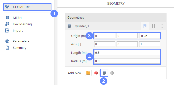
- Go to Geometry panel
- Select Create Cylinder
- 4 Define origin, length, and radius of the cylinder accordingly
Origin \({\sf [m]}\)00-0.25
Length \({\sf [m]}\)0.5
Radius \({\sf [m]}\)0.05
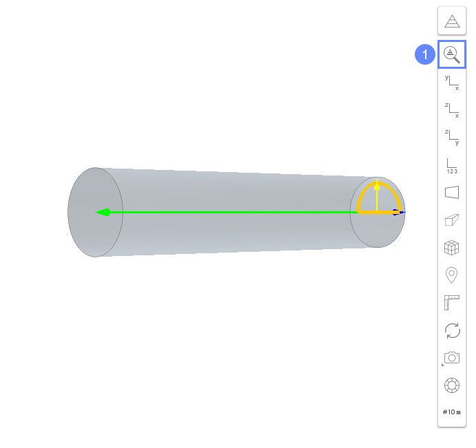
5. Geometry - Cylinder
After creating a cylindrical boundary, it will appear in the 3D panel.
- Click Fit View to zoom the geometry
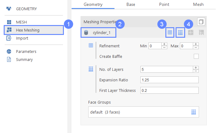
6. Meshing Properties - Cylinder
- Go to Hex Meshing panel
- Click cylinder_1
- Select Mesh Geometry
- Select Create Boundary Layer Mesh
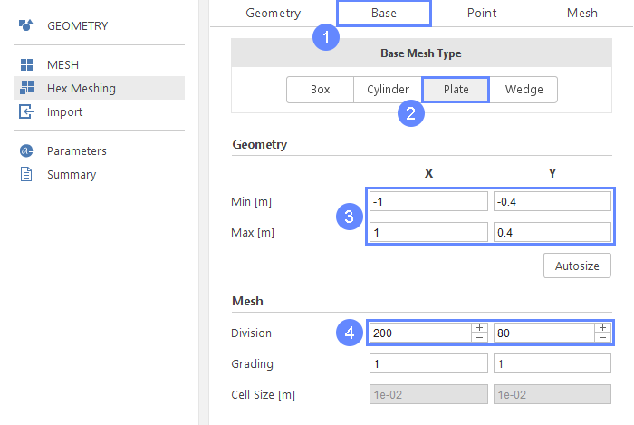
7. Base Mesh - Geometry and Mesh
We will define the base mesh now.
- Go to the Base tab
- Chose Plate Mesh Type
- Define base mesh minimum and maximum extend
Min \({\sf [m]}\)-1-0.4
Max \({\sf [m]}\)10.4 - Define division along each axis
Division200 80
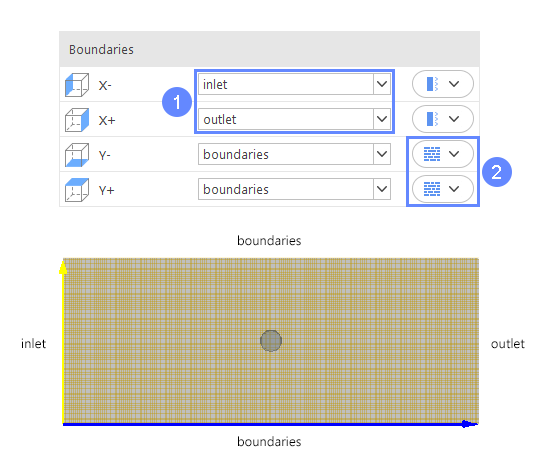
8. Base Mesh - Boundaries
- Define boundary names accordingly
X- inlet
X+ outlet - Define the following boundary types accordingly
Y- wall
Y+ wall
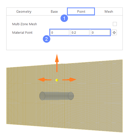
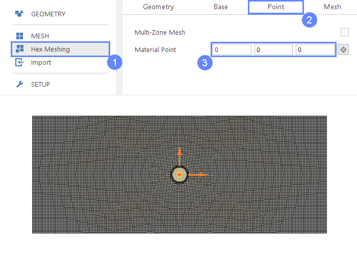
9. Material Point - Fluid
Now we will define material point outside the cylinder geometry.
- Go to Point tab
- Set location of the material point
Material Point00.20
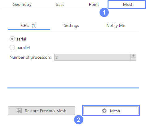
10. Meshing - Fluid Region
- Go to Mesh tab
- Start the meshing process with Mesh button

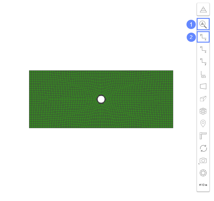
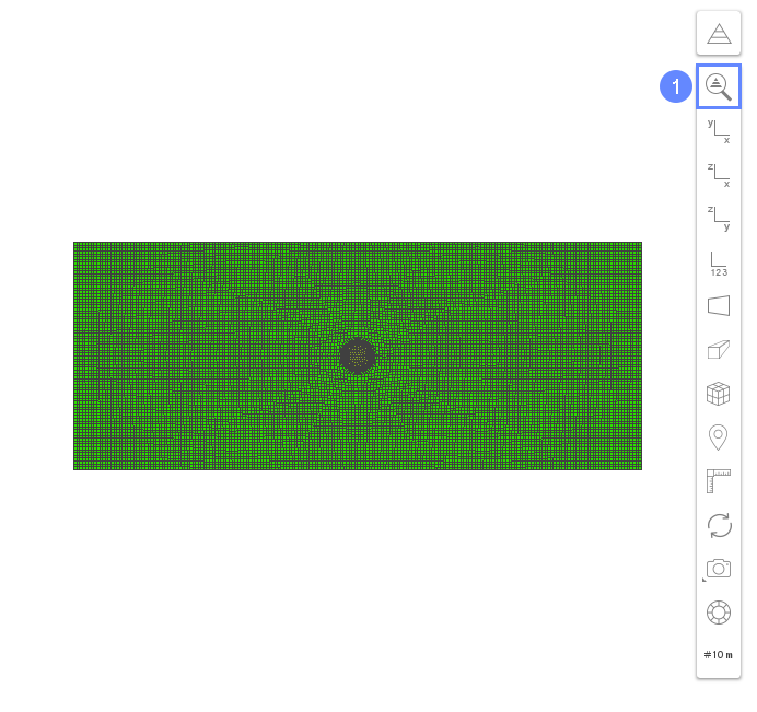
11. Mesh - Fluid Region
After a few minutes of meshing the following mesh should appear.
- Click Fit View to zoom the geometry
- Click View XY to orient view plane
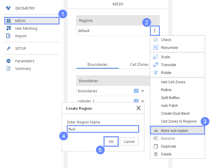
12. Create Sub-Region - Fluid
After creating the mesh, we have to make a sub-region - fluid.
- Go to Mesh panel
- Press Options button
- Select Make sub-region option
- Enter name fluid for the sub-region
- Click OK button
13. Material Point - Solid
Now we will define material point for sub-region - solid.
- Go to Hex Meshing panel
- Go to Point tab
- Set location of the material point
Material Point000
14. Meshing - Solid Region
Everything is set up now for the meshing of the solid region
- Go to Mesh tab
- Start the meshing process with Mesh button
15. Mesh - Solid Region
After a few minutes of meshing the following mesh should appear.
- Click Fit View to zoom the geometry
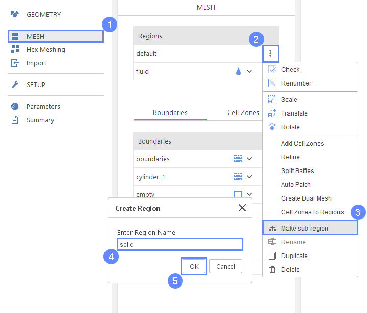
16. Create Sub-Region - Solid
After creating the mesh, we have to make a sub-region - solid.
- Go to Mesh panel
- Press Options button
- Select Make sub-region option
- Enter name solid for the sub-region
- Click OK button
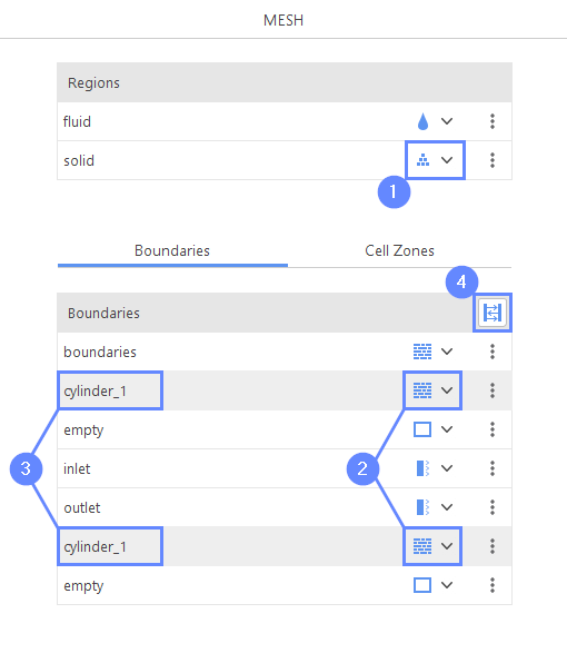
17. Create Region Interface
Two mesh regions are not coupled until you create a region interface. It will be further used to define which information is exchanged between regions.
- Select Solid type for solid region
- Make sure you have selected wall type for cylinder_1
- Hold CTRL key and select cylinder_1 in fluid and cylinder_1 in solid
- Click Create Region Interface icon
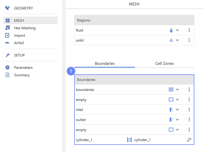
18. Check Mesh Boundaries
Verify the mesh by reviewing the boundary names and types.
- Ensure that each boundary is correctly named and assigned the appropriate type
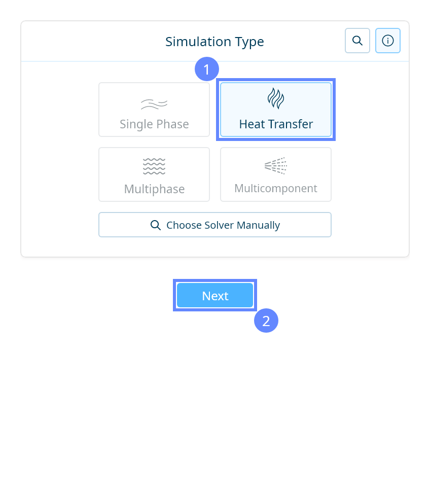
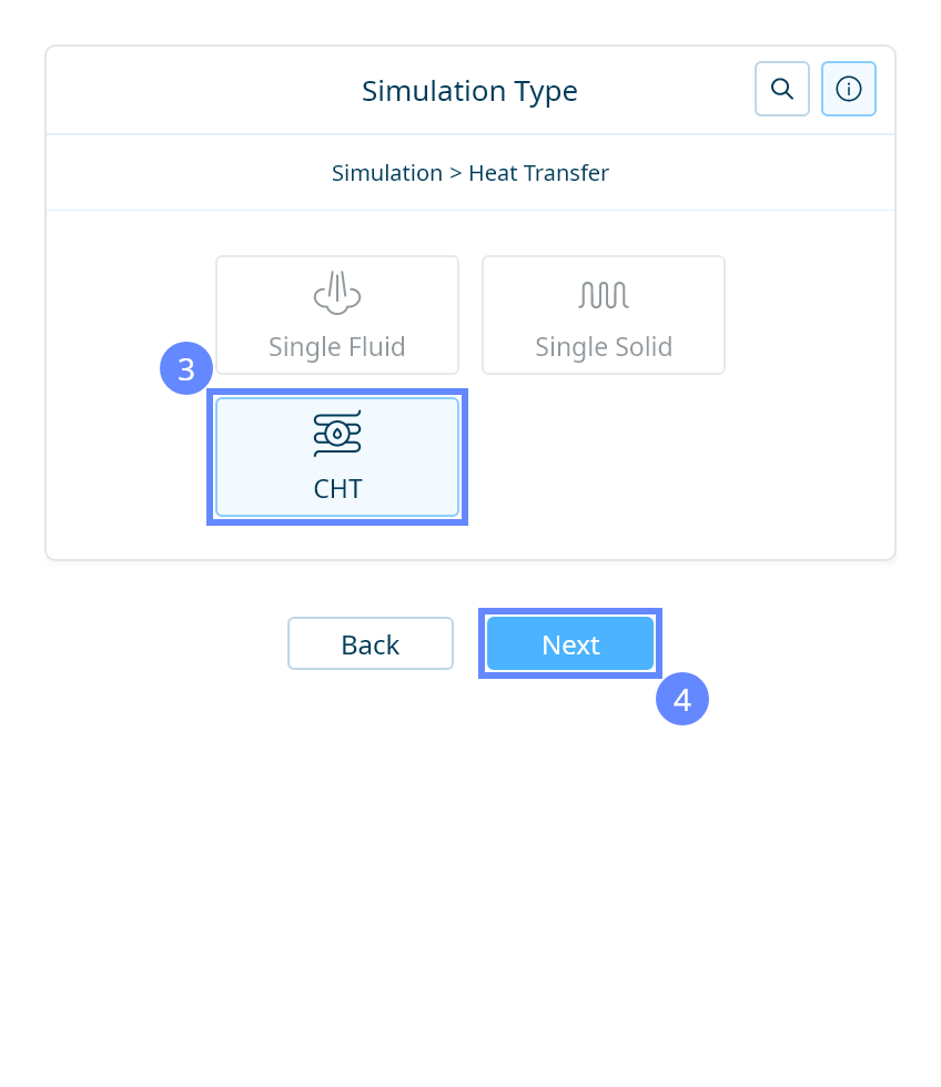
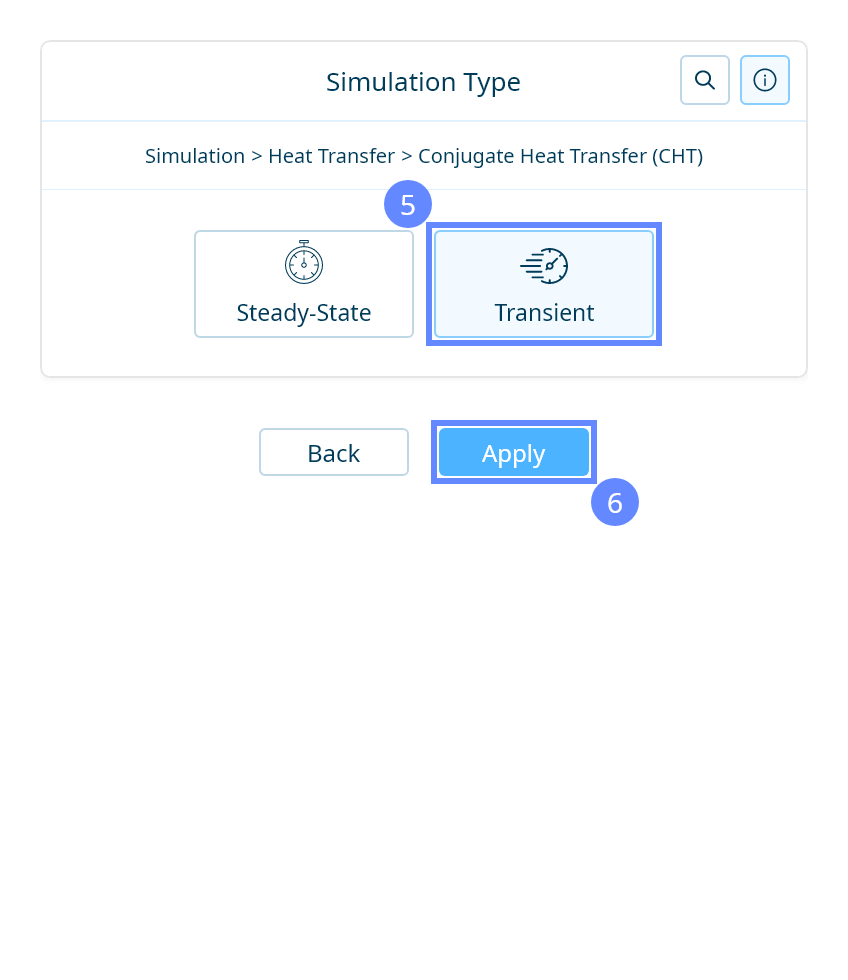
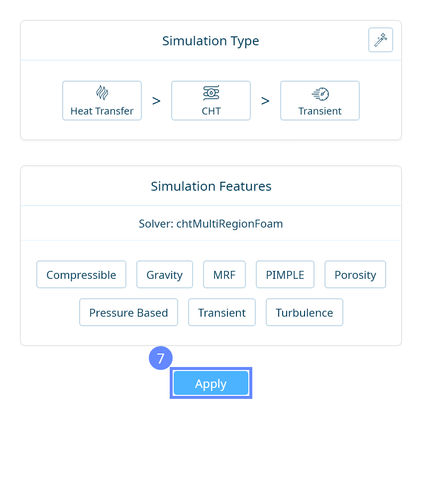
19. Simulation Type
We want to analyze a 2D simulation of a cooling cylinder. For this purpose, we will use a transient conjugate heat transfer simulation.

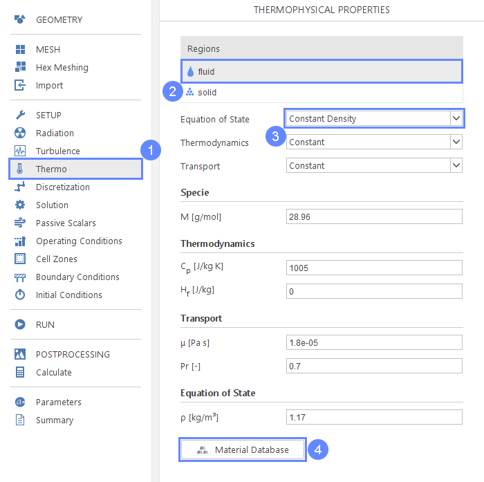
20. Thermophysical Properties - Fluid (I)
We will define now the thermodynamic properties of fluid material.
- Go to Thermo panel
- Select fluid region
- Select Constant Density
- Click Material Database button
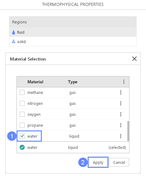
21. Thermophysical Properties - Fluid (II)
- Select water material
- Click Apply
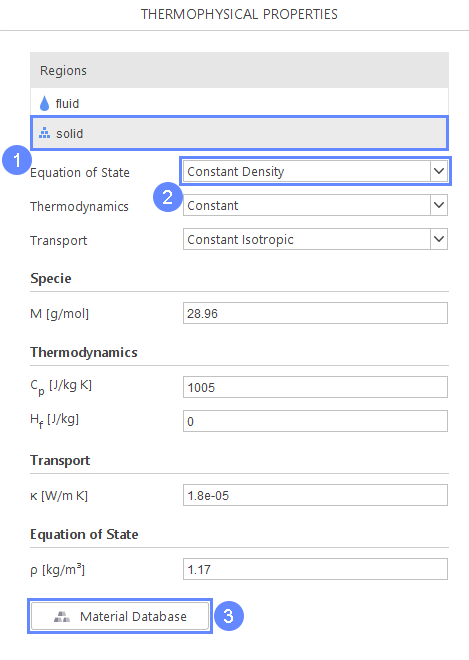
22. Thermophysical Properties - Solid (I)
We will define now the thermodynamic properties of solid material.
- Select solid region
- Select Constant Density
- Click Material Database button
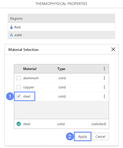
23. Thermophysical Properties - Solid (II)
- Select steel material
- Click Apply
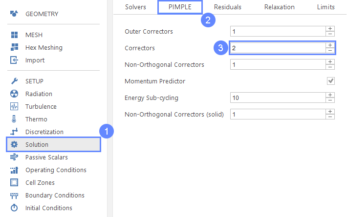
24. Solution - Solvers
- Go to Solution panel
- Go to the Pimple tab
- Increase the number of Correctors to 2
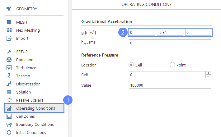
25. Operating Conditions
- Go to Operating Conditions panel
- Define gravitational acceleration
g \({\sf [m/s^2]}\)0-9.810
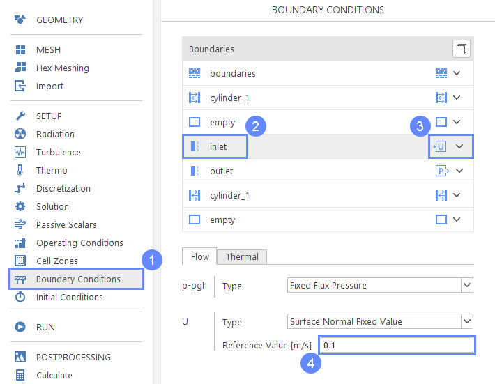
26. Boundary Conditions - Inlet (Flow)
- Go to Boundary Conditions panel
- Select inlet
- Change character to velocity inlet
- Define inlet velocity
Reference Value \({\sf [m/s]}\)0.1
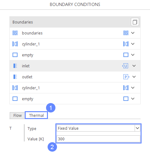
27. Boundary Conditions - Inlet (Thermal)
- Go to Thermal boundary conditions tab
- Set the following parameters accordingly
TypeFixed Value
Value \({\sf [K]}\)300
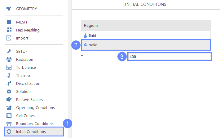
28. Initial Conditions
- Go to Initial Conditions panel
- Select solid region
- Set temperature T to 400
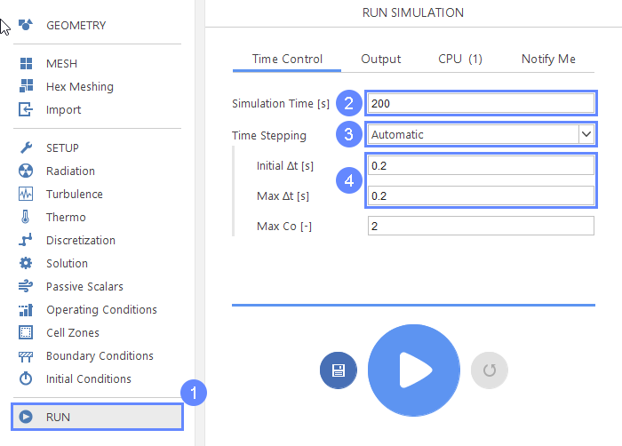
29. Run -Time Control
- Go to Run panel
- Set Simulation Time [s] to 200
- Change Time Stepping to Automatic
- Set initial and maximum time step accordingly
Initial \(\Delta t\) \({\sf [s]}\)0.2
Max \(\Delta t\) \({\sf [s]}\)0.2
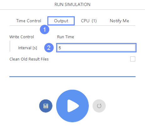
30. Run - Output
- Switch to Output panel
- Set Write Control Interval [s] to 5
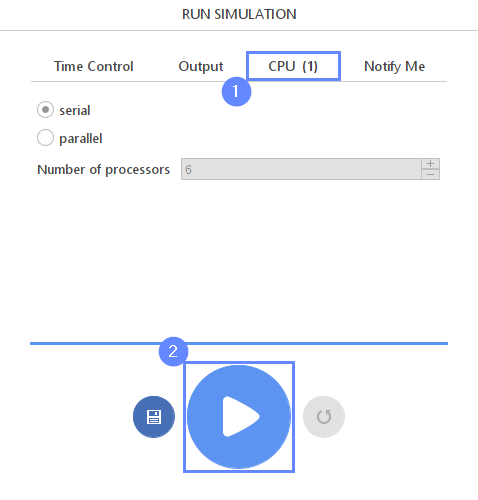
31. Run - CPU
To speed up the calculation process, take advantage of parallel computing and increase the number of CPUs based on your PC’s capability. The free version allows you to use only one processor (serial mode). To get the full version, you can use the contact form to Request 30-day Trial
Estimated computation time for serial mode: 5 minutes
- Switch to CPU tab
- Click Run Simulation button
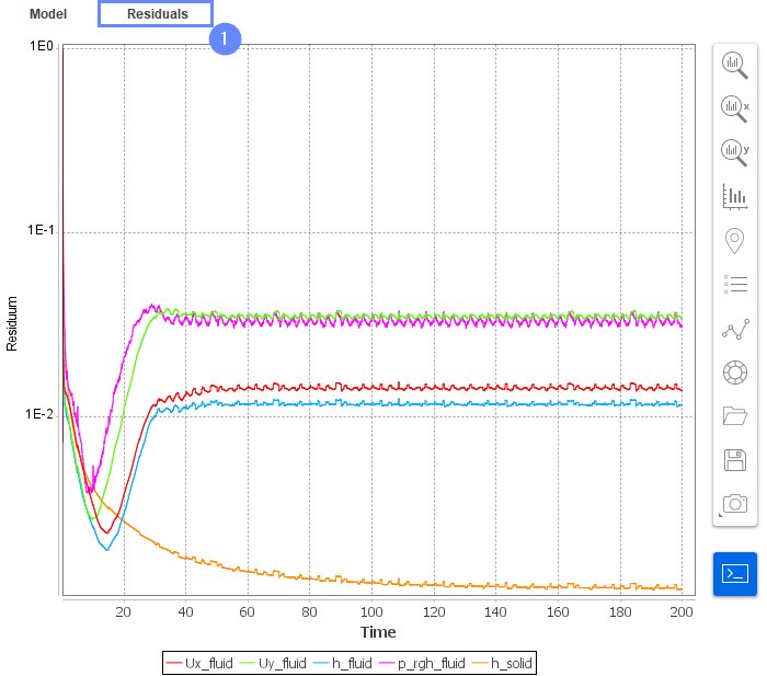
32. Residuals
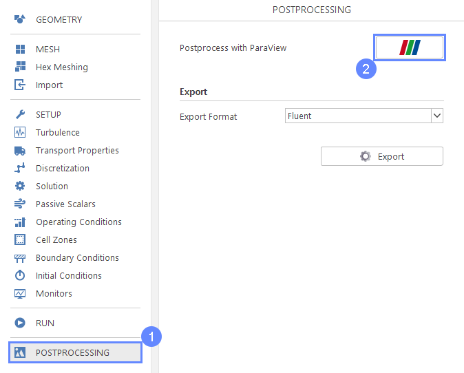
33. Start Postprocessing with ParaView
- Go to Postprocessing panel
- Run ParaView
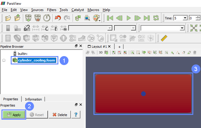
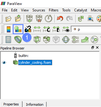
34. ParaView - Load Results
Now we are loading results into the ParaView.
- Select cylinder_cooling.foam
- Click Apply to load results into ParaView
- After loading results they will be shown in the 3D graphic window
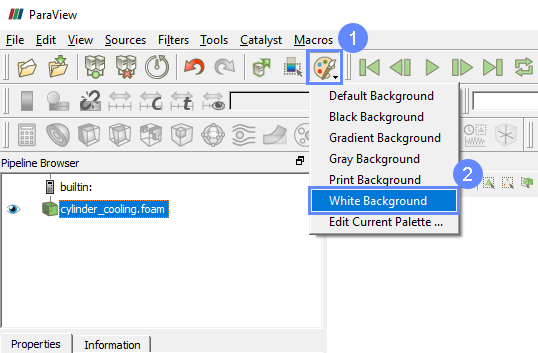
35. ParaView - Change Background
We can change the coloring scheme in ParaView to have nicer colors.
- Click Load a Color Palette
- Select White Background
36. ParaView - Choose Preset (I)
- Click Edit Color Map from the menu placed on the left side, if the panel is not already shown.
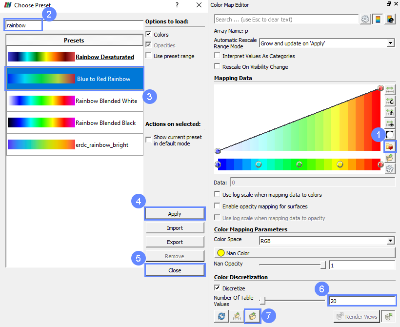
37. ParaView - Choose Preset (II)
- Select Choose Preset from the Color Map Editor placed by default on the right side of the ParaView
- Search rainbow
- Choose Blue to Red Rainbow preset.
- Apply changes
- Close Choose Preset window
- Set Number of Table Values to 20
- Click Save current color map settings values as default for all arrays
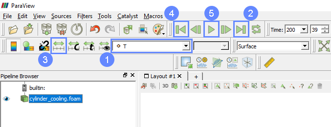
38. ParaView - Display Temperature Contour (I)
- Select contour coloring variable to T
- Click Last Frame
- Click Rescale to Data Range
- Click First Frame
- Click Play
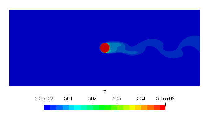
39. ParaView - Display Temperature Contour (II)
After applying changes the contour will be shown in the 3D window.
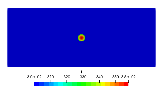
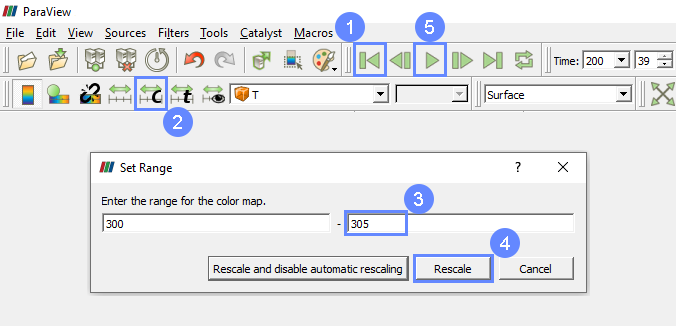
40. ParaView - Display Temperature Contour (III)
- Click First Frame
- Click Rescale to Custom Data Range
- Set maximum value
Max305 - Click Rescale
- Click Play
41. ParaView - Results