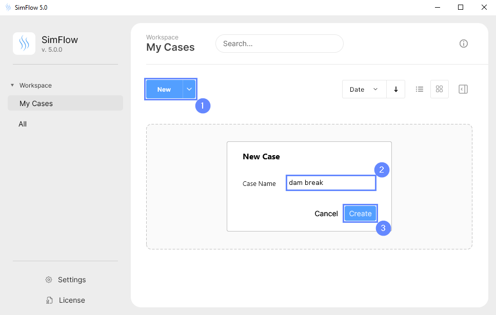
3. Create Case
Open SimFlow and create a new case named dam break
- Click New
- Provide name dam break
- Click Create to open a new case
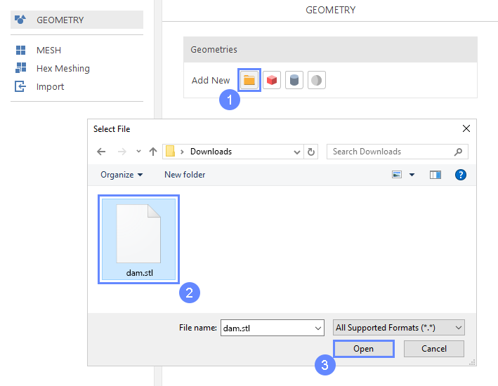
4. Import Geometry
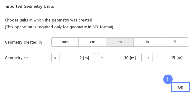
5. Imported Geometry Units
The STL geometry format does not store the unit in which the geometry was created. Geometry size shows the overall size of the model in each direction, which is helpful for unit selection. In our case, the default unit meter is correct.
- To confirm default unit meter, press OK
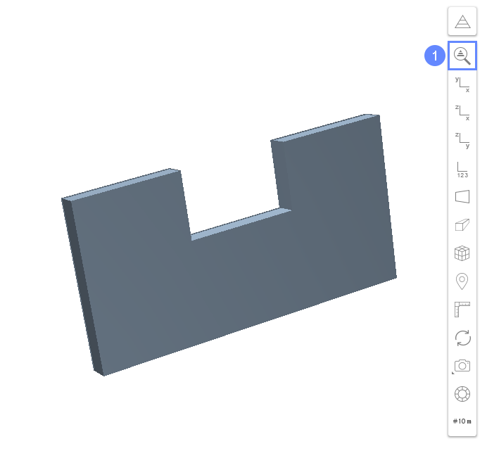
6. Geometry - Dam
After importing geometry, it will appear in the 3D panel.
- Click Fit View to zoom the geometry
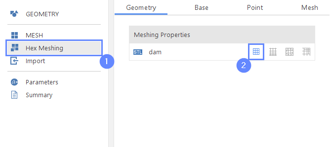
7. Enable Geometry Meshing
Now we need to enable meshing for the newly imported geometry.
- Go to Hex Meshing panel
- Enable meshing on the dam geometry
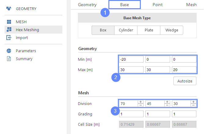
8. Base Mesh
Now we are going to define the computational domain in the Base Mesh panel.
- Go to Base tab
- Define initial mesh extends
Min \({\sf [m]}\)-2000
Max \({\sf [m]}\)303020 - Define mesh division
Division704530
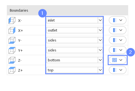
9. Base Mesh Boundaries
To define different boundary conditions on each side of the domain, you need to assign a unique name to each face of the base mesh. This will allow you to apply appropriate conditions later in the simulation setup.
- Assign boundary names from the dropdown list
X- inlet
X+ outlet - Manually type a custom name for the Y− face
Y- sides - Select boundary names for the remaining faces from dropdown list
Y+ sides
Z- bottom
Z+ top - Change the boundary type
Z- wall
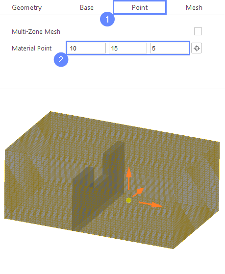
10. Material Point
We need to tell the meshing algorithm where the mesh should be retained.
- Go to Point tab
- Set coordinates of the material point
Material Point10155
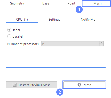
11. Start Meshing
Everything is now set up for meshing
- Go to Mesh tab
- Press Mesh button to start meshing process
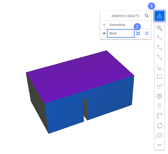
12. Mesh
After meshing process is finished the mesh will be loaded and displayed. To show what is inside of mesh, we can zoom in, or hide other meshes.
- Click Graphic Object List
- Select Mesh to show meshes list
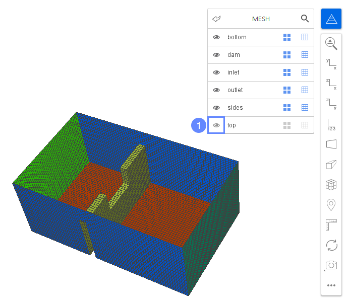
13. Mesh - Toggle Visibility
You can toggle the visibility of different objects to examine desired ones.
- Hide top boundary to look inside the mesh
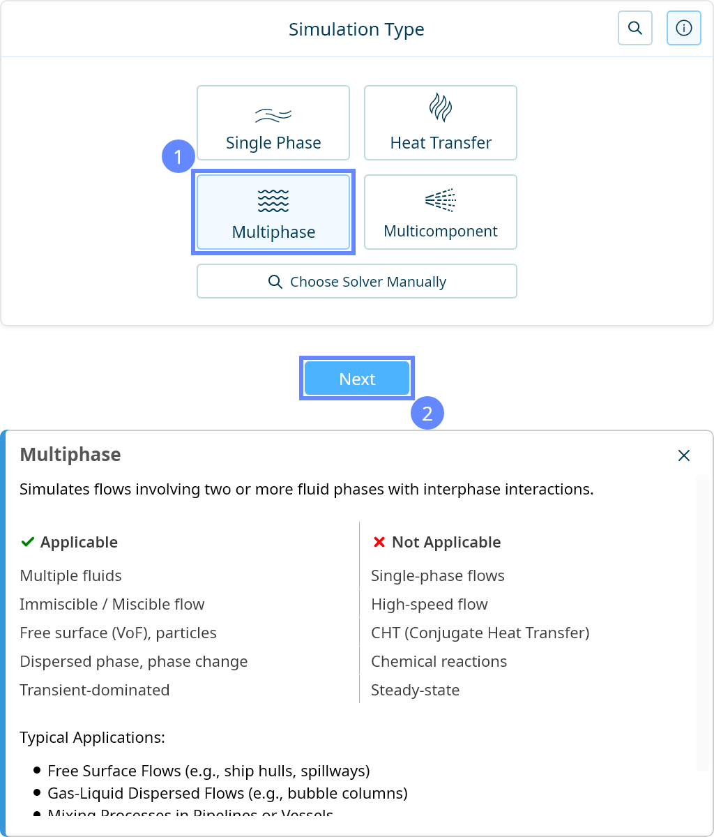
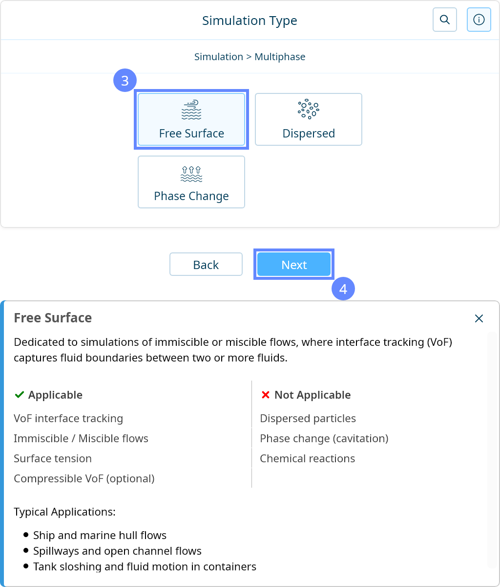
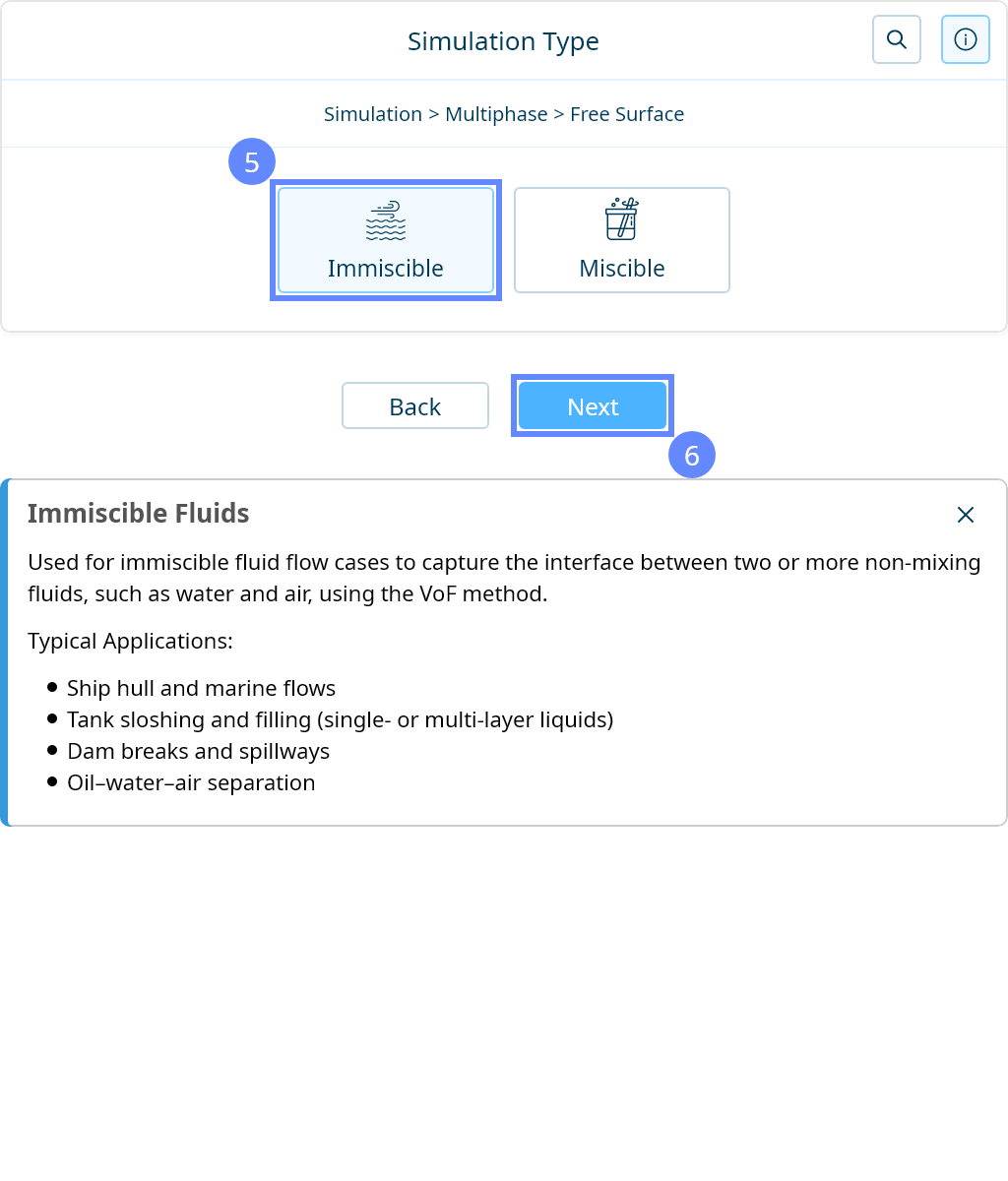
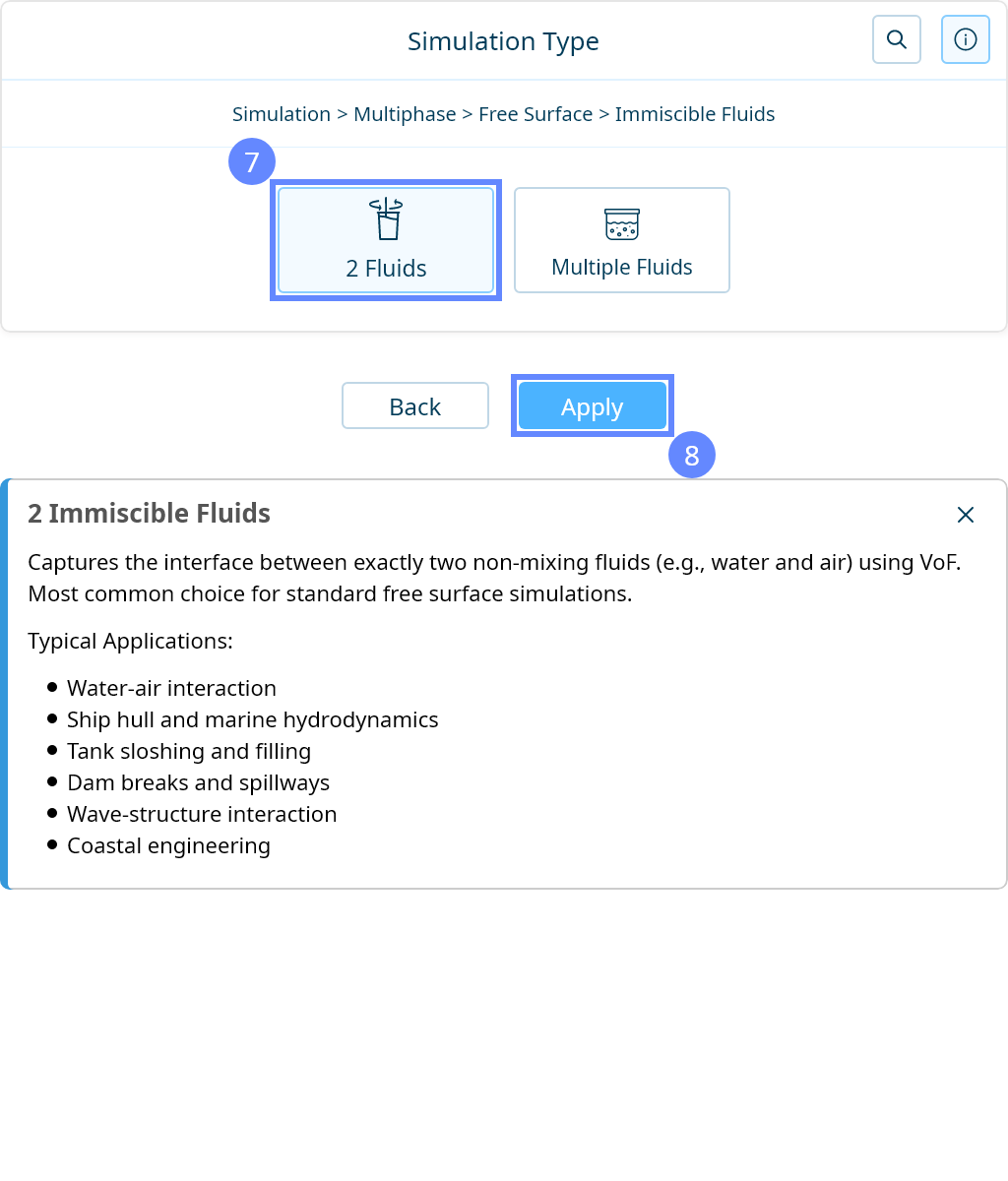
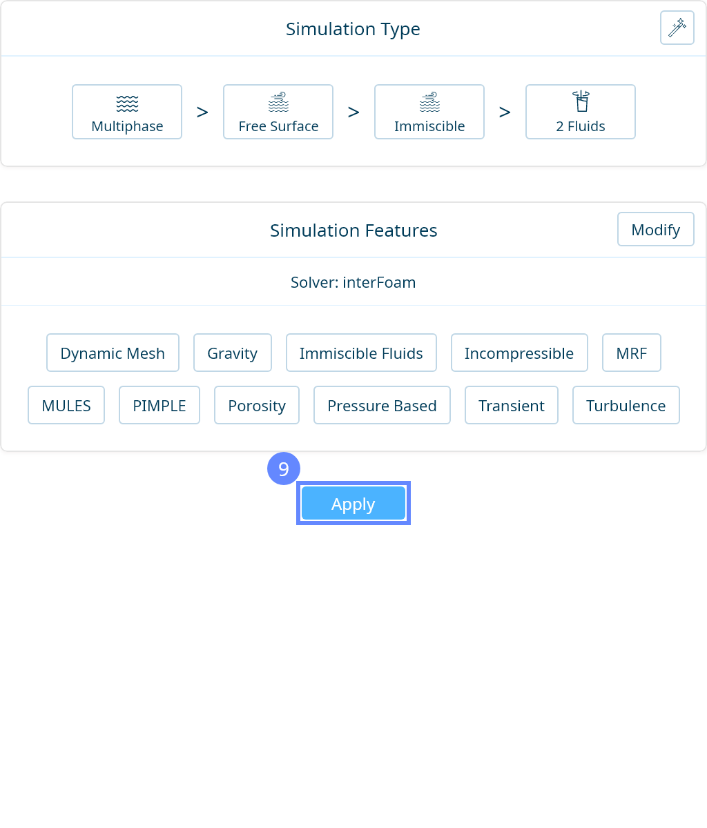
14. Simulation Type
We want to analyze water flow over a dam. For this purpose, we will use a transient simulation of two immiscible fluids (water and air) using the free-surface method.

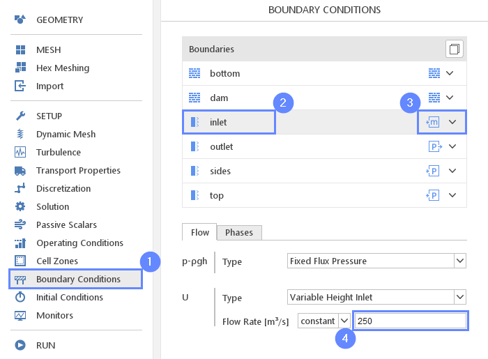
15. Boundary Conditions - Inlet (Flow)
At the inlet, we will apply a constant water flow rate in order to simulate water supplied by a river.
- Go to Boundary Conditions panel
- Select inlet boundary
- Set the Mass Flow Inlet character
- Set the mass flow rate
U Flow Rate \({\sf [m^3/s]}\)250
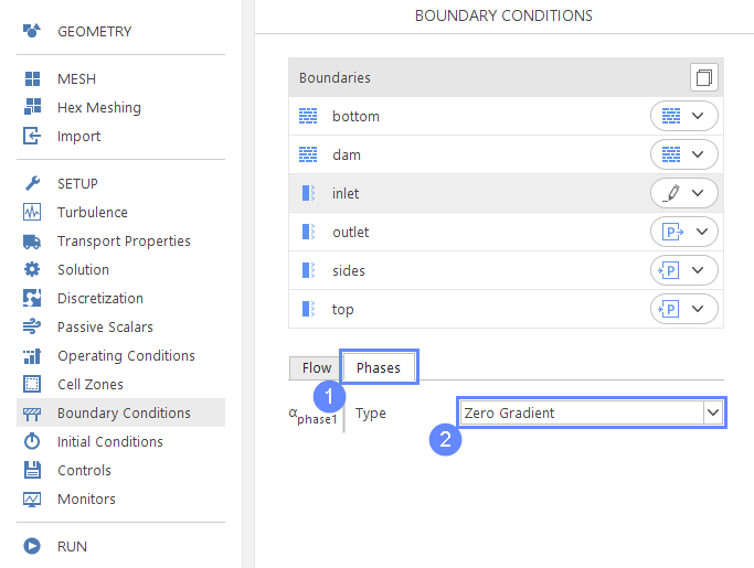
16. Boundary Conditions - Inlet (Phases)
We will modify the default phase fraction boundary condition to properly interact with the velocity boundary condition.
- Go to Phases tab
- Select the following boundary condition accordingly
\(\alpha_{phase1}\) TypeZero Gradient
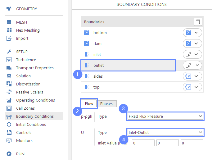
17. Boundary Conditions - Outlet (Flow)
On the outlet we want the water to freely flow out of the domain.
- Select outlet boundary
- Go to Flow tab
- 4 Set the following boundary conditions accordingly
\(p- \rho gh\) TypeFixed Flux Pressure
\(U\) TypeInlet-Outlet
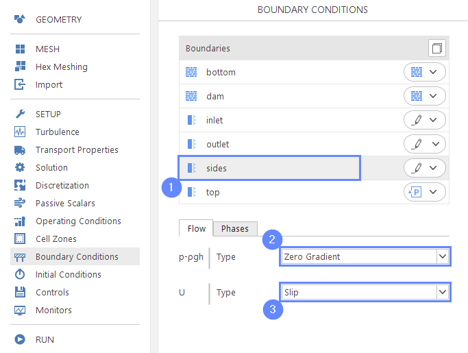
18. Boundary Conditions - Sides (Flow)
We want sides to be impermeable but did not provide any friction.
- Select sides boundary
- 3 Set the following boundary conditions accordingly
\(p- \rho gh\) TypeZero Gradient
\(U\) TypeSlip
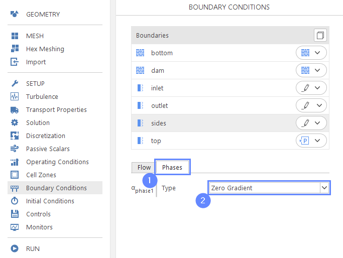
19. Boundary Conditions - Sides (Phases)
- Go to Phases tab
- Set the following boundary condition accordingly
\(\alpha_{phase1}\) TypeZero Gradient
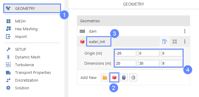
20. Geometry for Initialization
As an initial state, we want some water to already be behind the dam. For this purpose, we need to create geometry defining the initial location of water.
- Go to Geometry panel
- Create Box geometry
- Change name to water_init
- Define parameters accordingly
Origin \({\sf [m]}\)-2000
Dimensions \({\sf [m]}\)20309
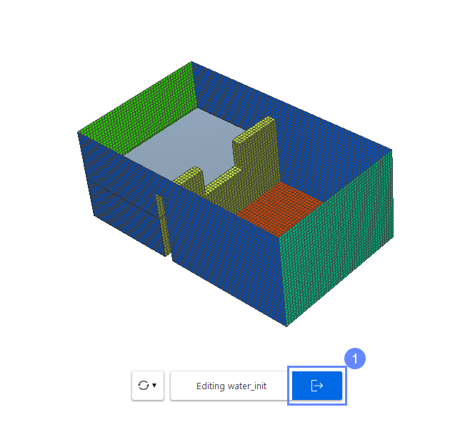
21. Geometry - Water Initialization
The gray box behind the broken dam geometry indicates the water we have created for the initialization part
- Exit edit mode and Deselect the geometry using buttons or by clicking Esc to have a proper view of the geometry
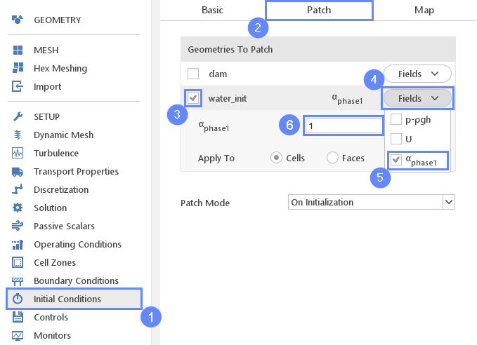
22. Initialization
We will use the water_init geometry to select the region where water phase fraction should be applied.
- Go to Initial Conditions panel
- Switch to Patch tab
- Enable initialization on water_init
- Expand Fields list
- Select \(\alpha_{phase1}\) fraction for initialization
- Set initial value of \(\alpha_{phase1}\) to 1
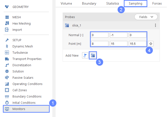
23. Slice Monitor (I)
Usually, we do data postprocessing when the computation is finished. However, it is handy to be able to see a preview of the results during the calculation. To do this, we need to use the Monitors panel where we might sample data in a specified point or section plane. In this tutorial, we will add a section plane, going through the center of our mesh.
- Go to Monitors panel
- Select Sampling tab
- Click on Create Slice button to enable sampling data on a section plane
- Set slice parameters accordingly
Normal \({\sf [-]}\)0-10
Point \({\sf [m]}\)81515.5
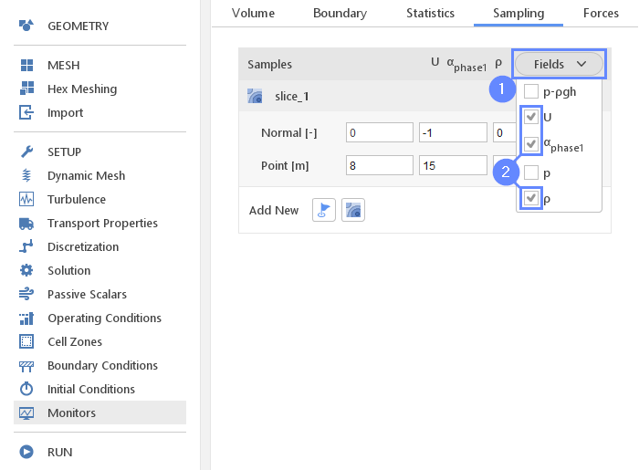
24. Slice Monitor (II)
Finally, we need to choose which data should be sampled on the section plane.
- Expand available Fields list
- Select \(U\), \(\alpha_{phase1}\) and \(\rho\)
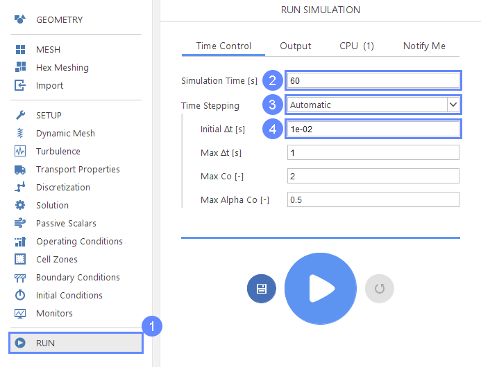
25. Run - Time Control
For multiphase simulations, we usually want the solver to automatically determine the proper time step. This should lead to good stability and reduce simulation time.
- Go to Run panel
- Specify simulation duration to 60 seconds
- Change Time Stepping to Automatic
- Set initial time step Initial \(\Delta t [s]\) to 1e-02
(solver will start computation with this value and adjust it in the next iterations)
In some situations, it might be necessary to use smaller time step values than the one provided by default configuration. To force solver reducing it you need to change the Max Co [-] (Courant Number). This property is used by the solver to automatically estimate the desired time step value.
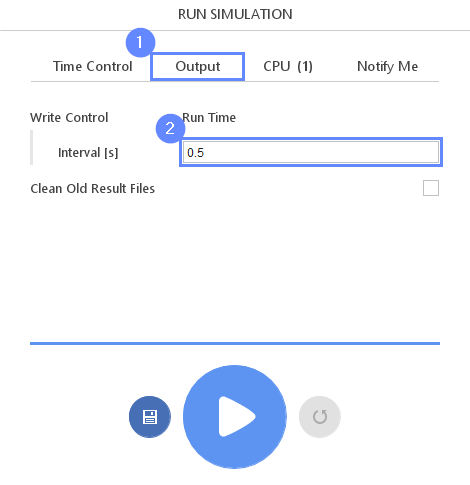
26. Run - Write Control
Before we will start computations we will specify intervals for writing data.
- Go to Output tab
- Set Write Control Interval [s] to 0.5 seconds
(The results will be written to the hard drive every 0.5 seconds of simulation time)
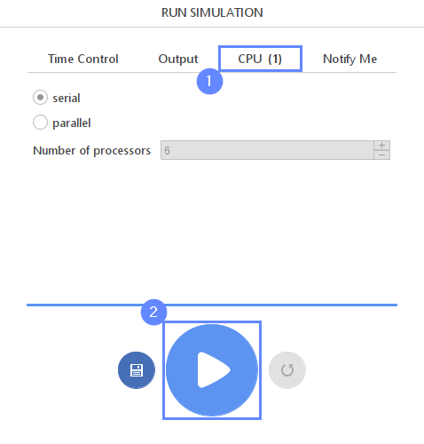
27. Run - CPU
To speed up the calculation process, take advantage of parallel computing and increase the number of CPUs based on your PC’s capability. The free version allows you to use only one processor (serial mode). To get the full version, you can use the contact form to Request 30-day Trial
Estimated computation time for serial mode: 35 minutes
- Switch to CPU tab
- Click Run Simulation button
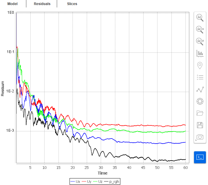
28. Residuals
When the calculation is finished we should see a similar residual plot.
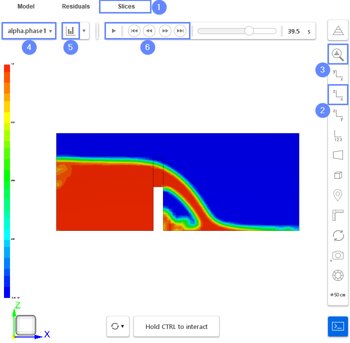
29. Preview Results on Slice
When the calculation is started SimFlow will automatically open the Residuals plots tab. When data is written to the disk for the first time new tab Slices will appear next to Residuals . Under this tab, we can preview results on the defined slice plane.
- Go to Slices tab
- Set the XZ orientation View XZ
- Click Fit View
- Select alpha.phase1 to display the location of the water phase
alpha.phase1 equal to 1 indicate water phase
alpha.phase1 equal to 0 indicate air phase - Click Adjust range to data
- Play with animation buttons to view the results of the analysis
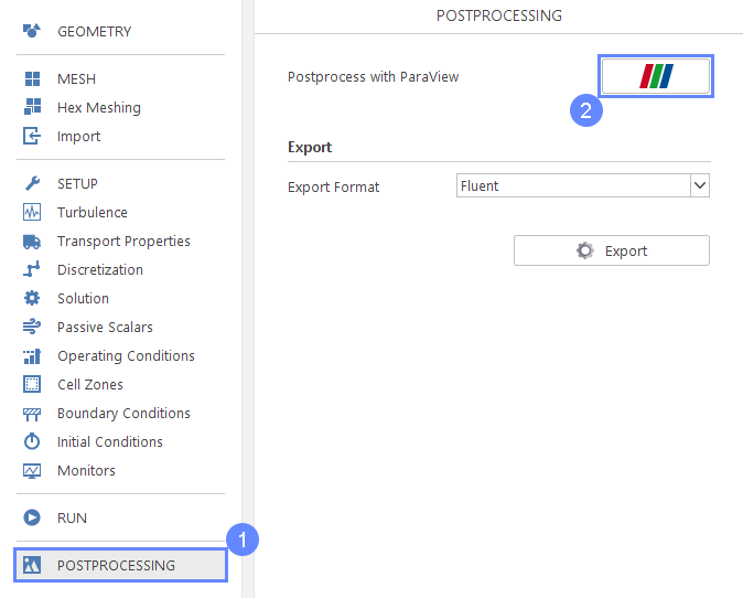
30. Postprocessing - ParaView
When the computations are finished start the ParaView software.
- Go to Postprocessing panel
- Start ParaView
You might also start ParaView when the simulation is still in progress to observe intermediate results
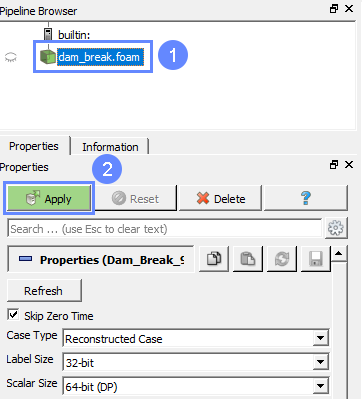
31. ParaView - Load Results
After opening the ParaView, we have to load the results of the simulation from SimFlow.
- Select your case
- Click Apply button to load results into ParaView
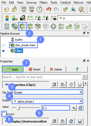
32. ParaView - Create Clip
We want to show how the water surface looks like. Additionally, we want the water surface to be colored based on the local velocity to better understand the flow behavior.
- Make sure your case is selected dam_break
- Create Clip
- Set Clip Type to Scalar
- Set Scalars to alpha.phase1
- Define water surface threshold Value to 0.2
- Make sure that Invert option is unchecked
- Apply changes
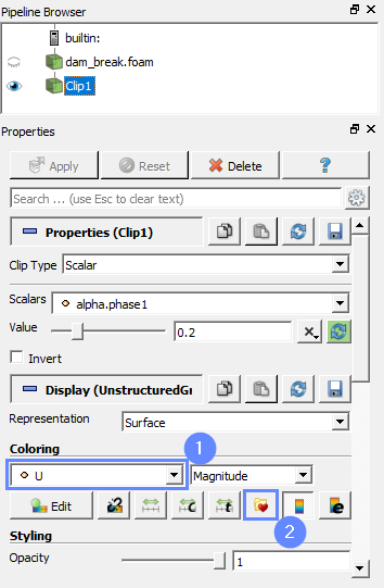
33. ParaView - Coloring
After the clip is created we can color water surface with velocity and choose color scale preset. While being still in the Properties panel.
- Select U (velocity) field
- Click Choose Preset button, a new window will appear (next step)
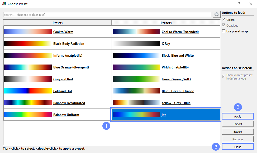
34. ParaView - Choose Preset
We can now select Color Preset of your choosing.
- Choose the jet preset.
- Apply changes
- Close Choose Preset window
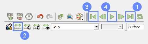
35. ParaView - Adjust Data Range and Play
- Change visible time step to Last Frame
- Fit colors range by clicking Rescale to Data Range
- Move to the First Frame
- Click Play to show simulation results
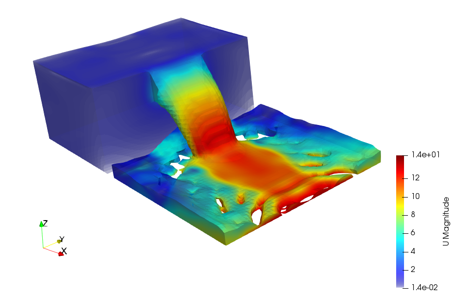
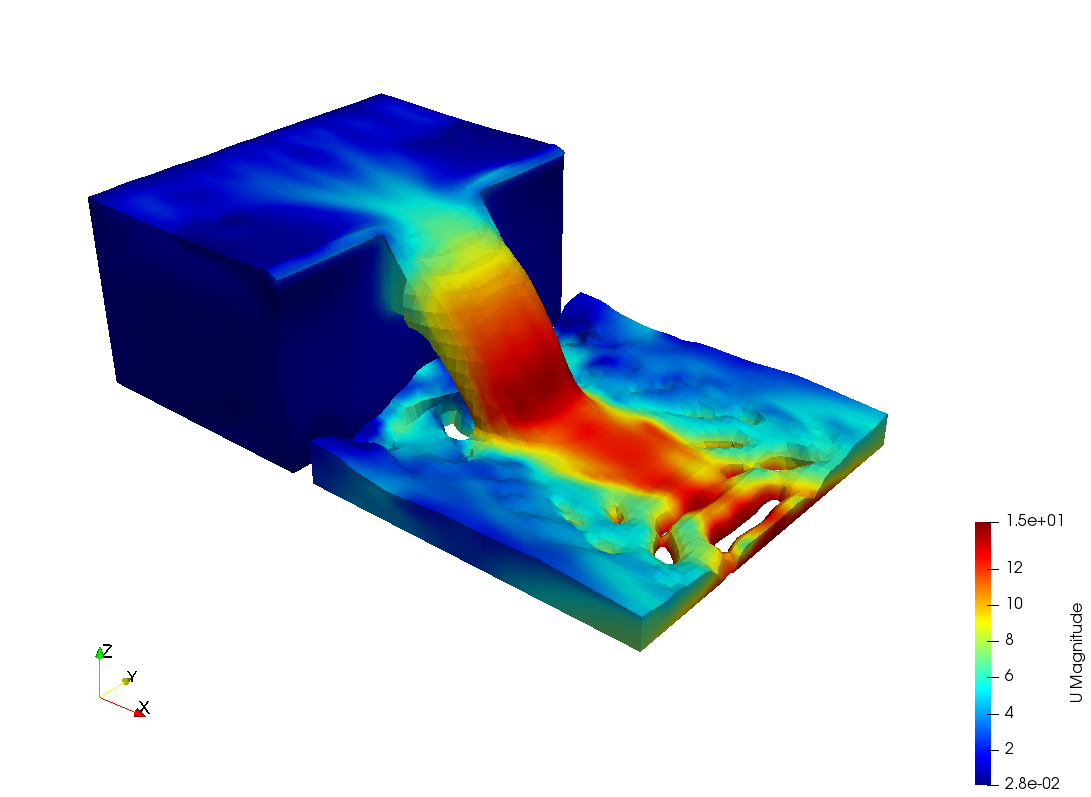
36. ParaView - Results
After correctly defining configuration you should be able to see similar results in the graphics 3D view.
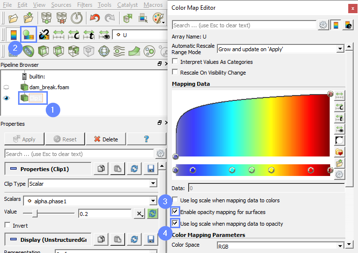
37. ParaView - Add Opacity
We can also add an opacity attribute to surface colors.
- Select Clip
- Click Edit if you do not see the Color Map Editor panel
- Check Enable opacity mapping for surfaces
- Check Use log scale when mapping data to opacity
38. ParaView - Results with Opacity