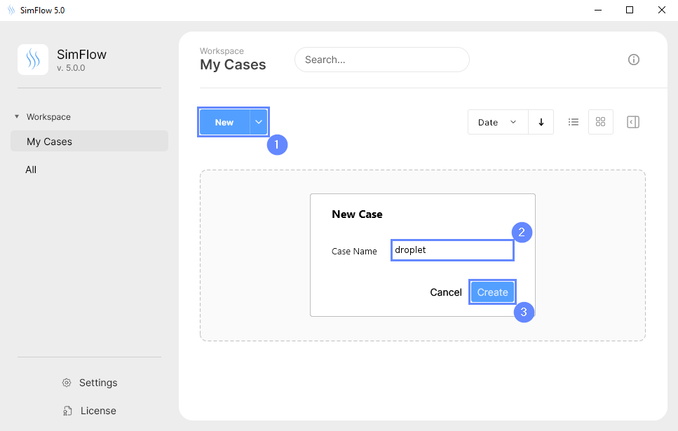
3. Create Case
Open SimFlow and create a new case named droplet
- Click New
- Provide name droplet
- Click Create to open a new case
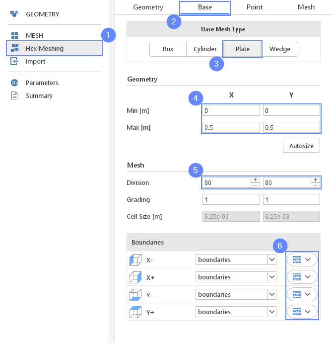
4. Meshing parameters
We will start by creating a 2D mesh. This can be accomplished by choosing the Plate type as the background mesh.
- Go to
Hex Meshingpanel - Go to
Basetab - Select
Plateas aBase Mesh Type - Define minimum and maximum extend
Min \({\sf [m]}\)00 - Define the number of divisions
Division8080 - Change boundary type to
wallfor all background mesh boundaries
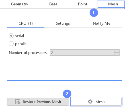
5. Start Meshing
We will start by creating a 2D mesh. This can be accomplished by choosing the Plate type as the background mesh.
Now we are ready to create our simple mesh.
- Go to
Meshtab - Press the Mesh button to start meshing process
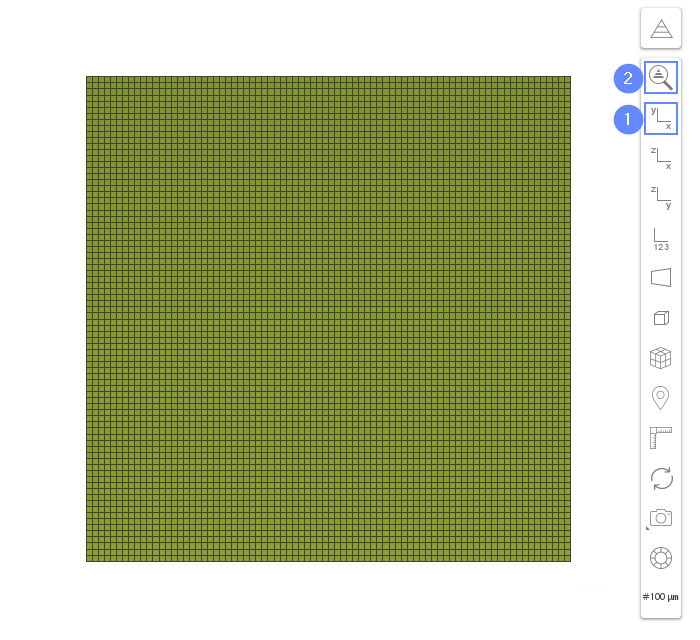
6. Mesh
After the meshing process is finished, the mesh should appear in the graphics window.
- Click ViewXY or press CTRL+F1 to orient view plane
- Click Fit View to zoom the geometry
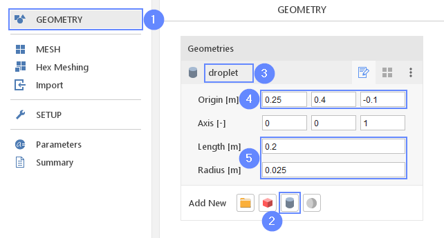
7. Create Geometry - Droplet
To indicate the initial shape of the droplet we will use cylinder geometry.
- Go to
Geometrypanel - Select Create Cylinder
- Change geometry name from
cylinder_1to droplet - Set the origin
Origin \({\sf [m]}\)0.250.4-0.1 - Set the cylinder dimensions
Length \({\sf [m]}\)0.2
Radius \({\sf [m]}\)0.025
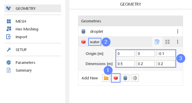
8. Create Geometry - Water
Additionally, we would like the droplet to fall down into the tank partially filled by water. To fill the bottom part of the domain with the water we will add another geometry.
- Add a new geometry by clicking Create Box
- Change geometry name from
box_1to water - Set the origin and box dimensions
Origin \({\sf [m]}\)00-0.1
Dimensions \({\sf [m]}\)0.50.20.2
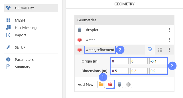
9. Create Geometry - Water Refinement
To be able to better resolve water behavior, we will create an area with a higher mesh resolution. To do this, we will add two more box geometries.
- Select Create Box
- Change geometry name from
box_1to water_refinement - Set the origin and box dimensions
Origin \({\sf [m]}\)00-0.1
Dimensions \({\sf [m]}\)0.50.30.2
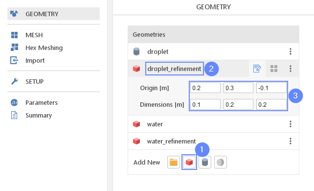
10. Create Geometry - Droplet Refinement
The second refinement box will be located at the path of the falling droplet.
- Select Create Box
- Change geometry name from
box_1to droplet_refinement - Set the origin and box dimensions
Origin \({\sf [m]}\)0.20.3-0.1
Dimensions \({\sf [m]}\)0.10.20.2
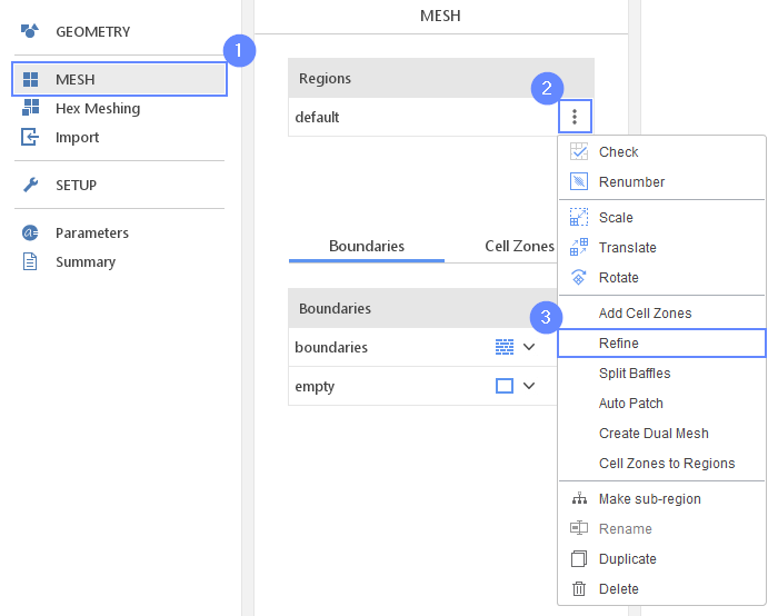
11. Refine Mesh (I)
- Go to
Meshpanel - Expand the
Optionslist next todefaultregion - Select
Refine
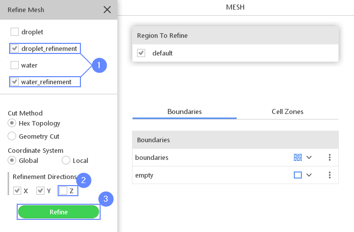
12. Refine Mesh (II)
- Check the refinement regions
droplet_refinement
water_refinement - Uncheck the Z axis in
Refinement Directions - Click Refine
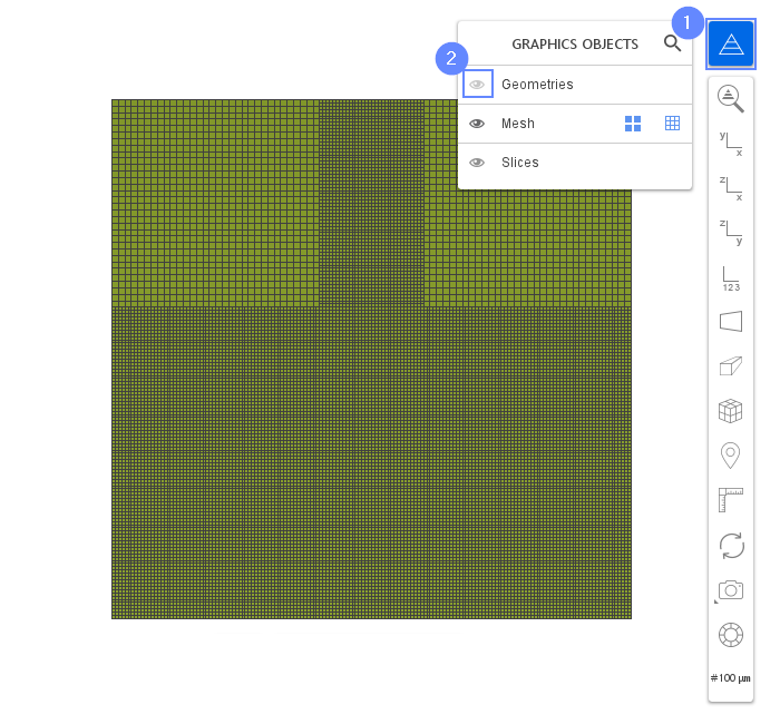
13. Display Mesh
Check the refinement region by hiding the geometries and displaying mesh.
- Click Graphic Object List
- Uncheck
Geometry
To hide the Graphics Objects panel press the Esc key. |
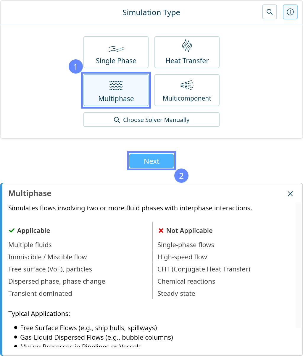
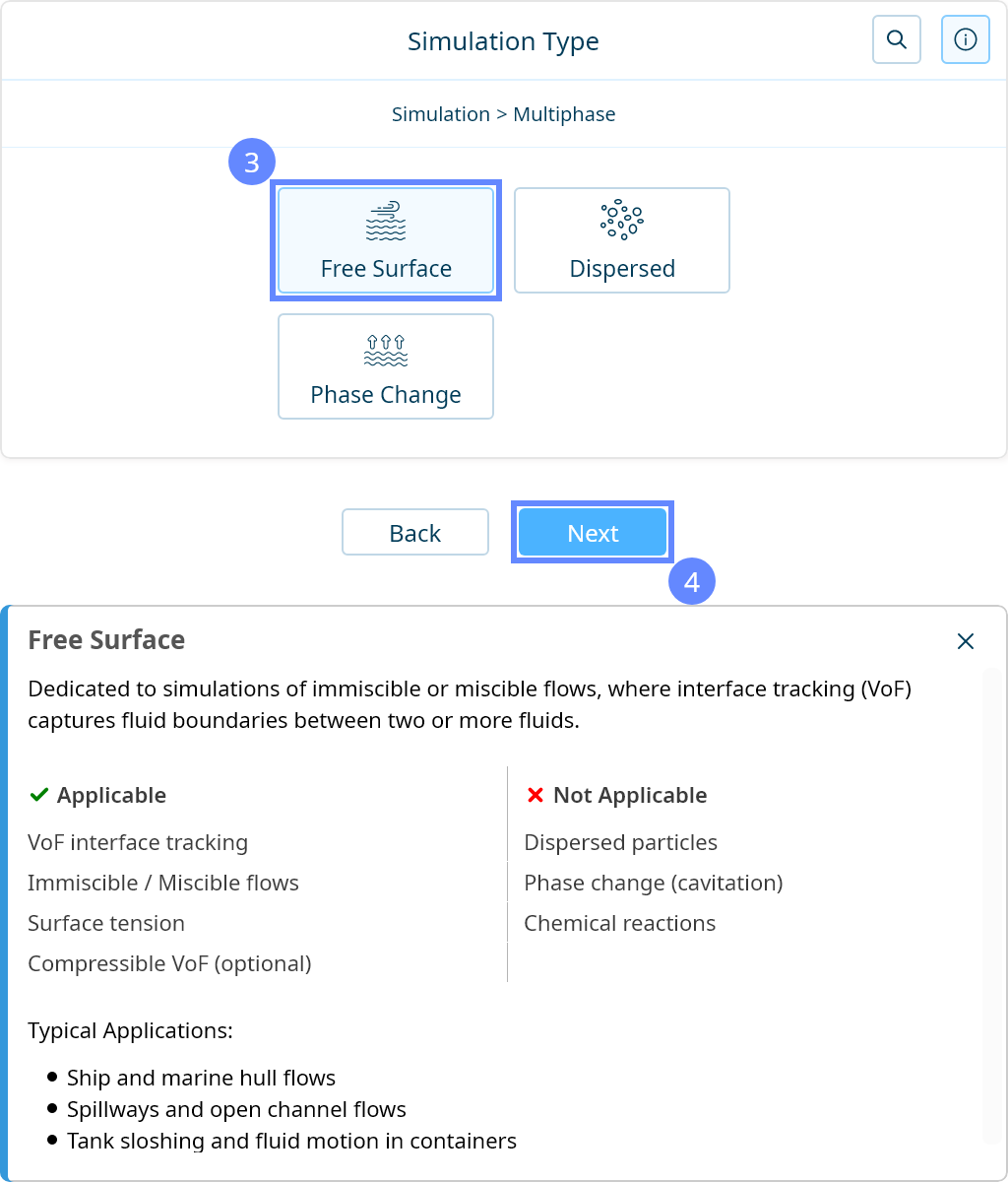
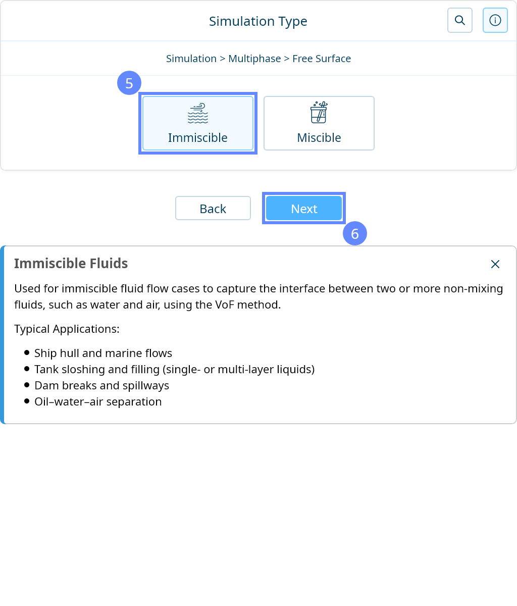
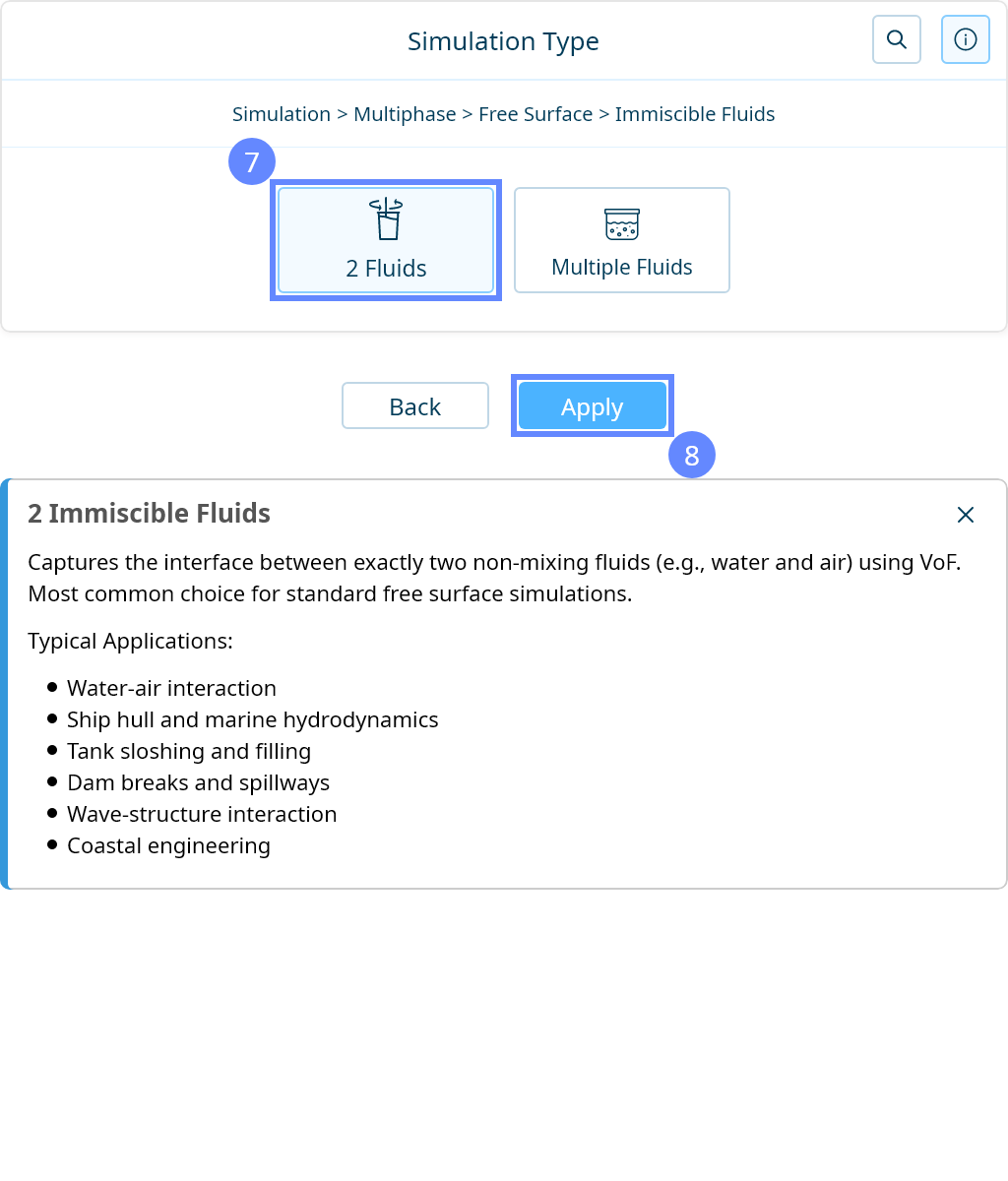
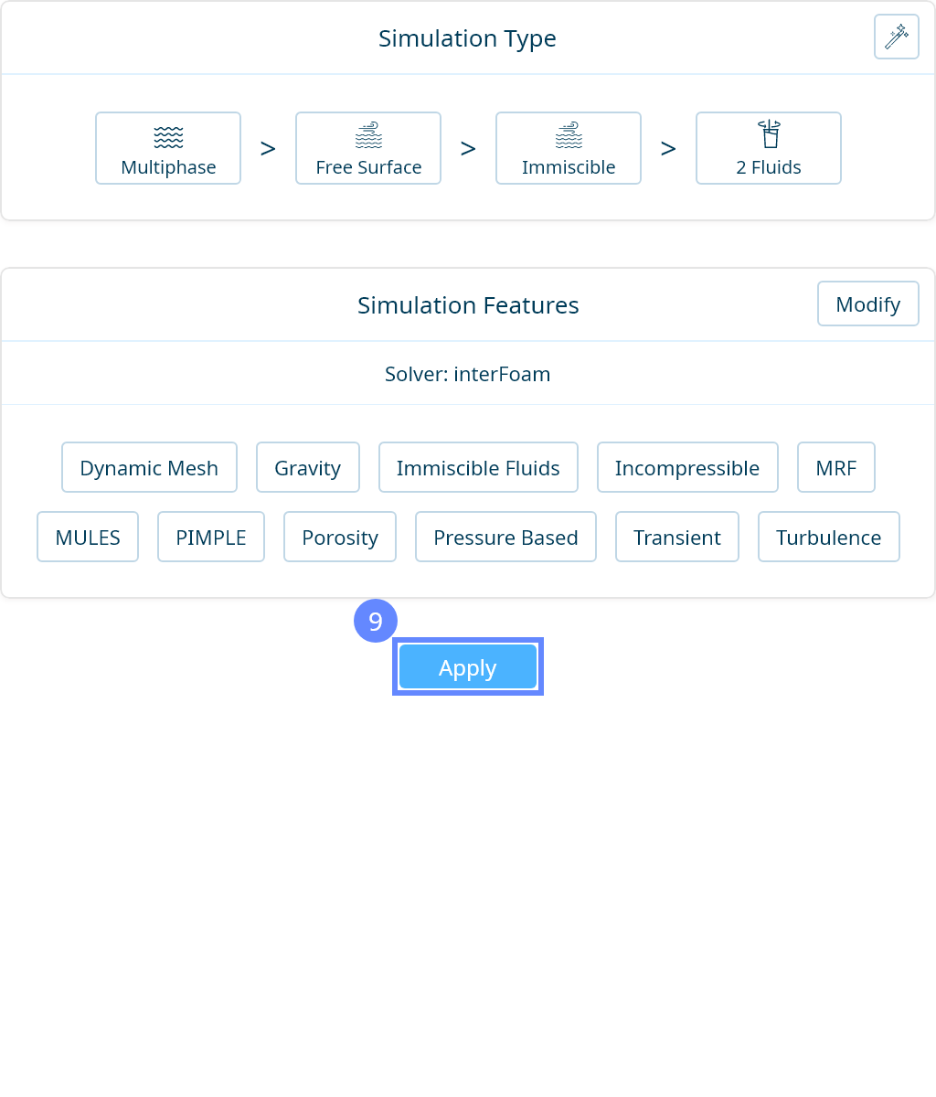
14. Simulation Type
We want to analyze the behavior of a water droplet. For this purpose, we will use a transient simulation of two immiscible fluids (water and air) using the free-surface method.

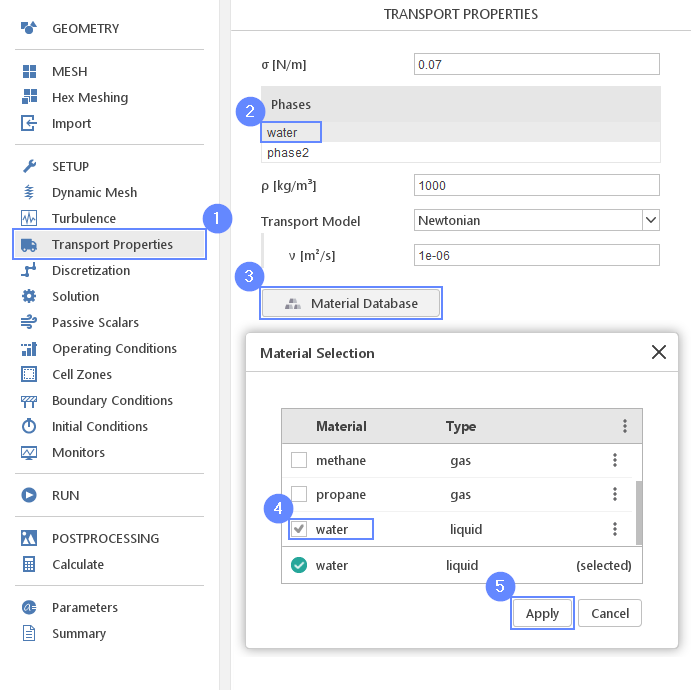
15. Transport Properties - Water
Now we will define the transport properties for both fluids.
- Go to
Transport Propertiespanel - Change phase name from
phase1to water - Open Material Database
- Pick up
waterfrom the list - Click Apply
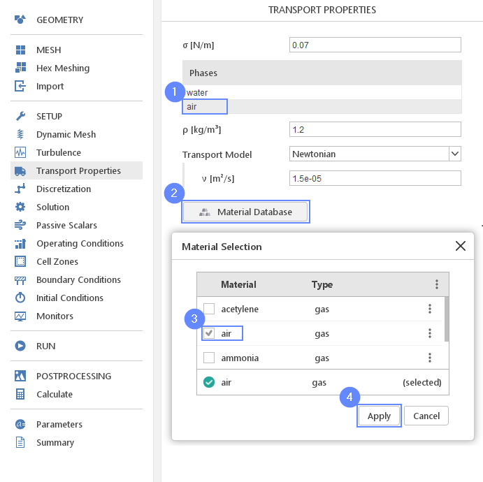
16. Transport Properties - Air
Repeat this step for phase2 using air properties.
- Change phase name from
phase2to air - Open Material Database
- Pick up
airfrom the list - Click Apply
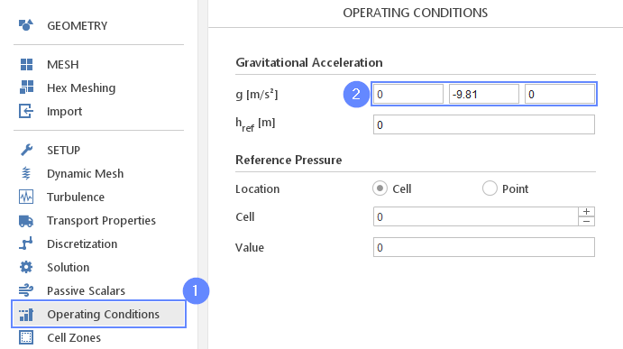
17. Operating Conditions - Gravity
- Go to
Operating Conditionspanel - Define gravitational acceleration along negative Y-axis
g \({\sf [m/s^2]}\)0-9.810
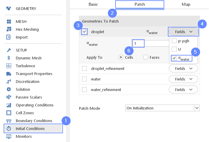
18. Initial Conditions - Droplet
We will use the droplet geometry to select the region where water phase fraction should be initially applied.
- Go to
Initial Conditionspanel - Switch to
Patchtab - Enable initialization on
droplet - Expand Fields list
- Select \(\alpha_{water}\) fraction for initialization
- Set initial value of \(\alpha_{water}\) to 1
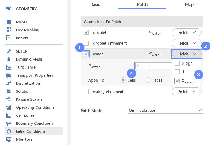
19. Initial Conditions - Water
Repeat the step for water geometry.
- Enable initialization on
water - Expand Fields list
- Select \(\alpha_{water}\) fraction for initialization
- Set initial value of \(\alpha_{water}\) to 1
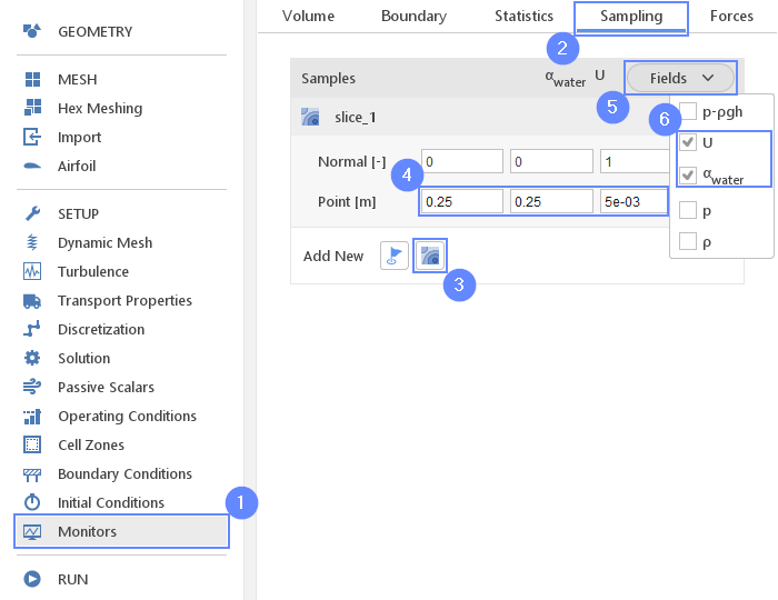
20. Monitors - Create Slice
During calculation, we can observe intermediate results on a section plane. To add sampling data on a plane we need to define plane properties and also select variables that will be sampled. Note that runtime post-processing can only be defined before starting calculations and can not be changed later on.
- Go to
Monitorspanel - Switch to
Samplingtab - Select Create Slice
- Set the origin to
Point \({\sf [m]}\)0.250.255e-03 - Expand Fields list
- Check U and \(\alpha_{water}\)
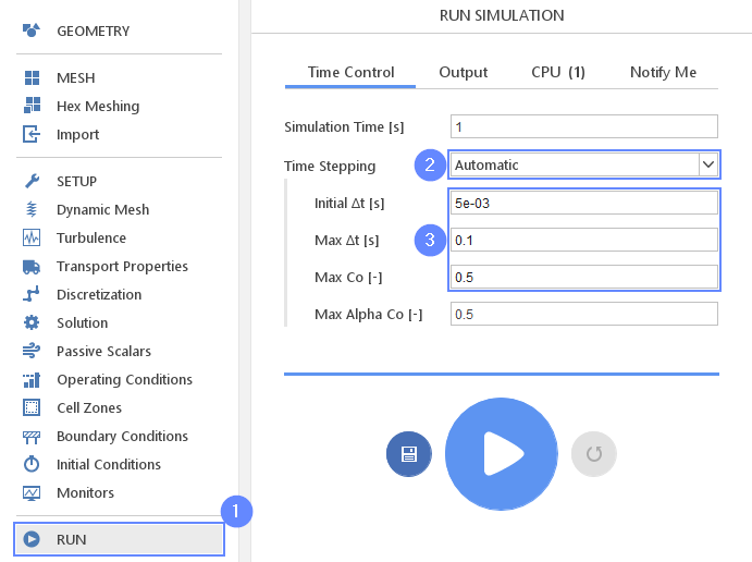
21. Run - Time Controls
For any simulation, it is very convenient to let the solver automatically determine the proper time step value. To use this option we need to define time step constraints by providing the initial time step(adjusted by the solver during computations), maximal time step value and the Courant number. In our case, we will reduce the default Courant number for better stability and quality.
- Go to
RUNpanel - Change
Time SteppingtoAutomatic - Set initial time step, time step limit and Courant number accordingly
Initial \(\Delta t\) \({\sf [s]}\)5e-03
Max \(\Delta t\) \({\sf [s]}\)0.1
Max Co \({\sf [-]}\)0.5
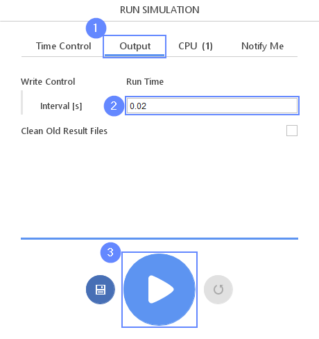
22. Run - Output
It is very important to control when results should be stored on the hard drive. This is especially important for the transient simulations where users are interested in the whole flow history saved as a collection of the snapshots.
- Switch to
Outputtab - Set
Write ControlInterval [s]to 0.02
(solver will store results on the hard drive every 0.02 second of the simulation) - Click Run Simulation button
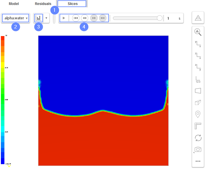
23. Results
When calculations will begin SimFlow automatically will switch view to the Residuals tab, where we can observe the convergence of our simulation. This is very handy for steady-state simulations when we try reaching low residuals levels. In case of transient simulation, we would rather like to see how our flow develops as simulation time progress.
- Switch to
Slicestab - Choose alpha.water field
- Click Adjust range to data
- Play with an animation buttons to track the results of analysis