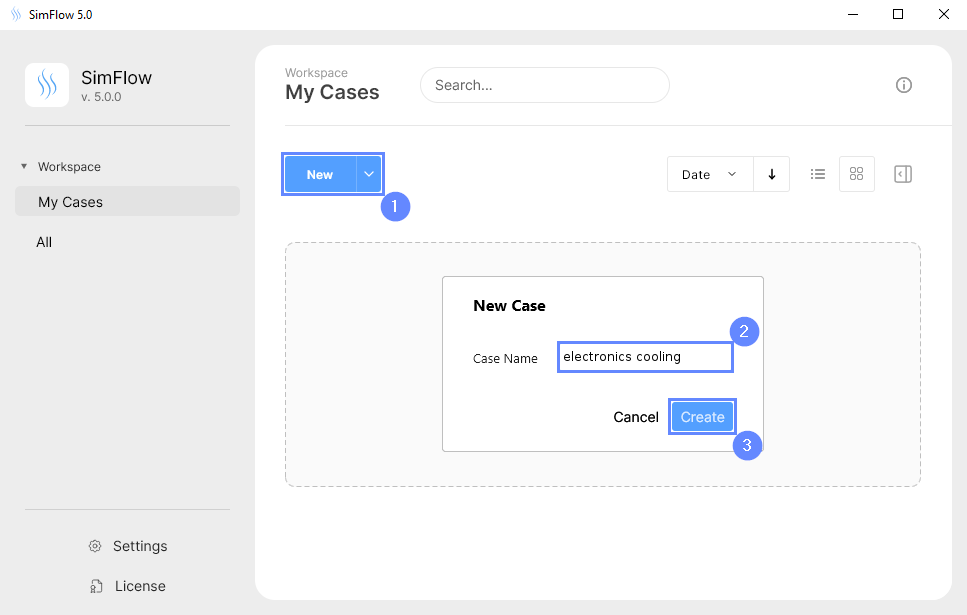
3. Create Case
Open SimFlow and create a new case named electronics cooling
- Click New
- Provide name electronics cooling
- Click Create to open a new case
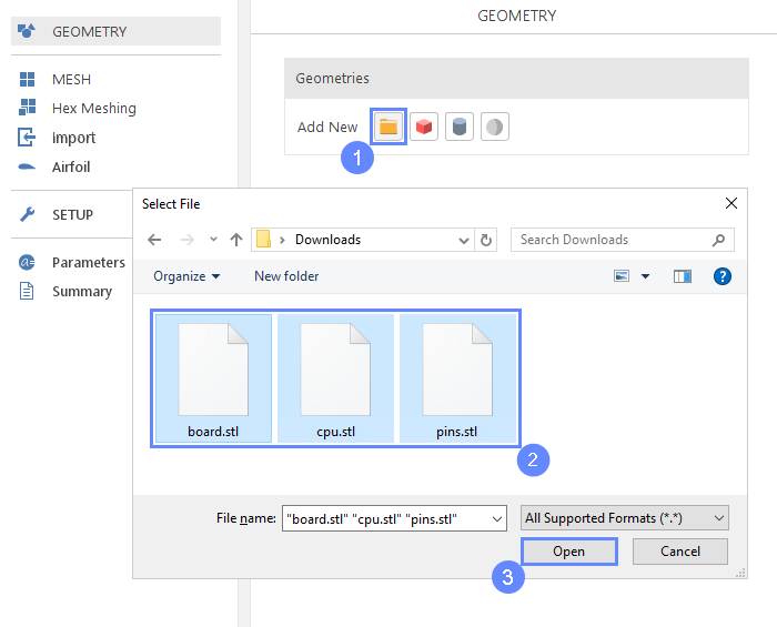
4. Import Geometry
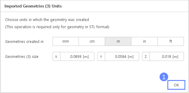
5. Imported Geometry Units
The imported geometry is in STL format, which does not store unit information. We need to confirm the unit in which the model was created. In the selection of unit, we can use the Geometry size label, which displays overall size of the model in each direction. In our case, the default unit meter is correct.
- To confirm default unit meter, press OK
6. Display Geometry
After loading geometry, it will appear in the graphics window
- Click Fit View button to zoom out the geometry
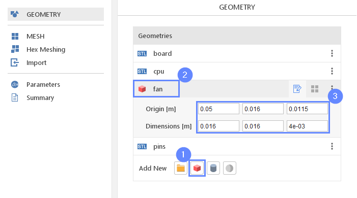
7. Create Geometry - Fan
Add fan geometry to the model. It will be placed above the CPU.
- Select Create Box
- Change geometry name from box_1 to fan
(double click to edit name and press Enter to confirm) - Set the origin and box dimensions
Origin \({\sf [m]}\)0.050.0160.0115
Dimensions \({\sf [m]}\)0.0160.0164e-03
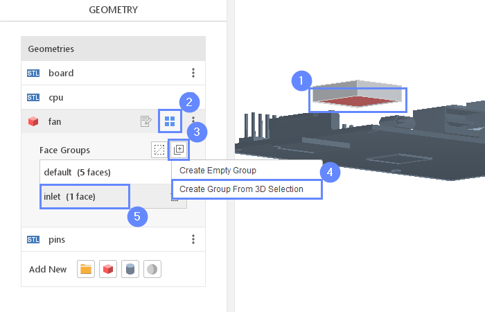
8. Create Face Groups - Fan Inlet
Now rotate the geometry of the model so that we can see the bottom side of the newly created fan. We will now select a face that will be subdivided from the fan as a separate boundary patch by the meshing tool.
- Press Ctrl and select this bottom surface of the fan
- Click Geometry Faces next to fan
- Click Create New Face Group
- Click Create Group From 3D Selection
- Rename group_1 to inlet
(double click on the group to rename, press Enter to confirm)
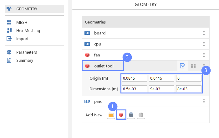
9. Create Geometry - Outlet Tool
The last primitive geometry to create is a box that will be used as a tool to extract outlet patch from outer boundaries
- Select Create Box
- Change geometry name from box_1 to outlet_tool
- Set the origin and box dimensions
Origin \({\sf [m]}\)0.08450.04150
Dimensions \({\sf [m]}\)6.5e-039e-038e-03
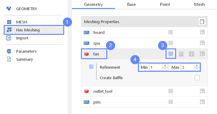
10. Meshing Parameters - Fan
Since we are going to perform CHT (Conjugate Heat Transfer) simulation, we need to create the mesh for fluid and solid sub-domains. We will specify the mesh parameters for all geometries and using the material point we will choose the subdomain that will be meshed.
- Go to Hex Meshing panel
- Select fan geometry
- Enable Mesh Geometry
- Set Refinement to Min 1 Max 3
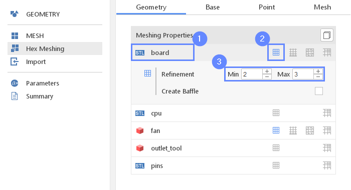
11. Meshing Parameters - Board
- Select board geometry
- Enable Mesh Geometry
- Set Refinement to Min 2 Max 3
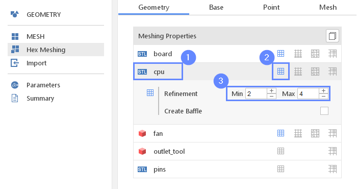
12. Meshing Parameters - CPU
- Select cpu geometry
- Enable Mesh Geometry
- Set Refinement to Min 2 Max 4
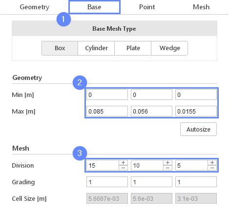
13. Base Mesh - Domain
Now, we will define the base mesh. The box geometry determines the background mesh domain.
- Go to Base tab
- Define the box size
Min \({\sf [m]}\)000
Max \({\sf [m]}\)0.0850.0560.0155 - Define the number of divisions
Division15105
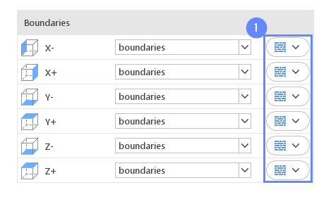
14. Base Mesh Boundaries
- Change boundary type to wall for all base mesh boundaries
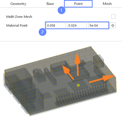
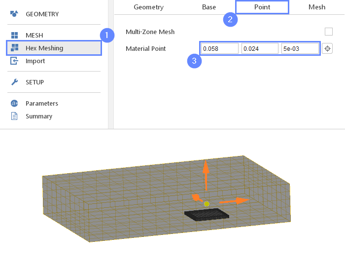
15. Solid Mesh - Material Point
In order to create the mesh in the solid region, we will place the material point inside the fan geometry. The resulting mesh will remain only in this region.
- Go to Point tab
- Specify location inside the CPU box
Material Point0.0580.0245e-04
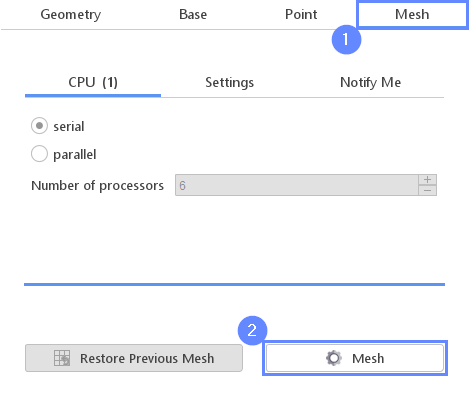
16. Solid Mesh - Start Meshing
Everything is set up now for the meshing of the solid region
- Go to Mesh tab
- Press Mesh button to start meshing process
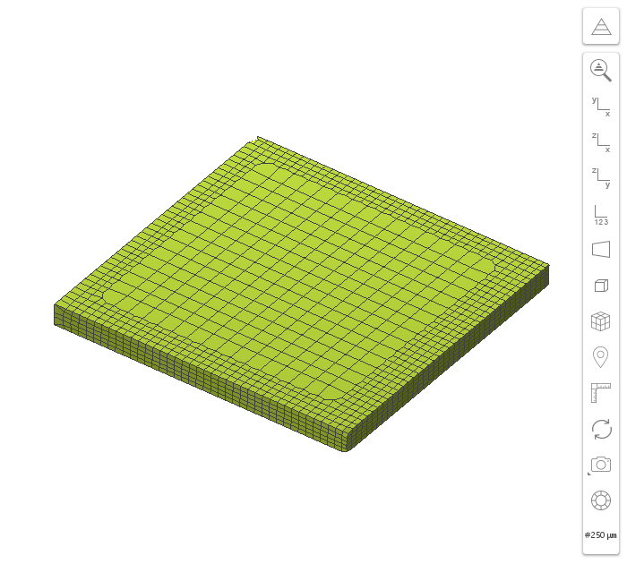
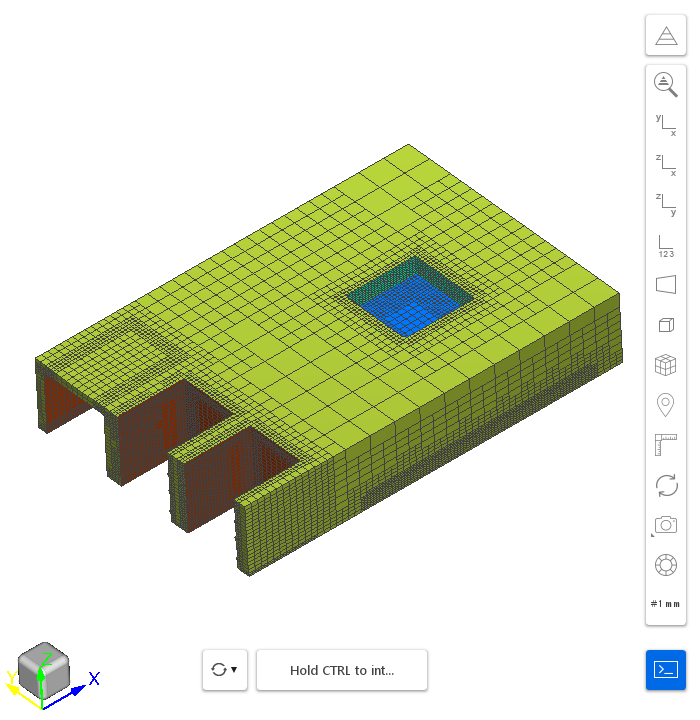
17. Solid Mesh
When the meshing process is finished, the solid region mesh appears on the screen.
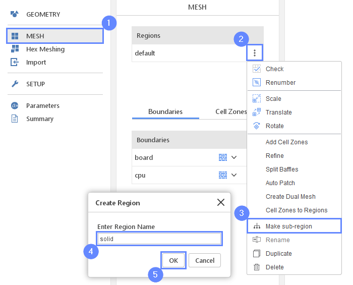
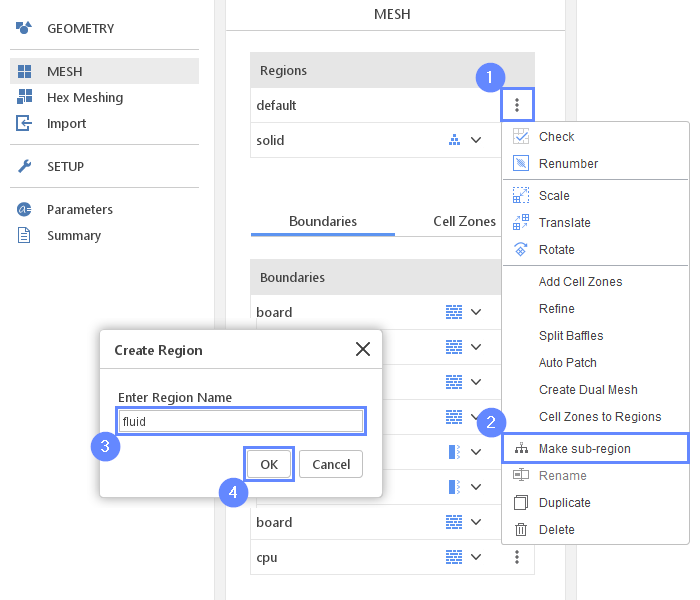
18. Solid Mesh - Create Sub-region
Before generating a mesh for the fluid region, you must convert the current mesh into a sub-region. Otherwise, it would be overwritten by the new mesh.
- Go to MESH panel
- Expand the Options list next to the default region
- Select Make sub-region
- Enter Region Name to solid
- Press OK
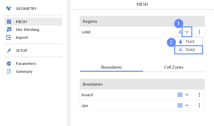
19. Solid Mesh - Type
- Expand region type options
- Select Solid
20. Fluid Mesh - Material Point
Once the solid region is created, we can move the material point to anywhere inside the base mesh, but outside the solid region.
- Go to Hex Meshing panel
- Go to Point tab
- Specify location inside the fluid mesh
Material Point0.0580.0245e-03
21. Fluid Mesh - Start Meshing
Everything is set up now for the meshing of the fluid region
- Go to Mesh tab
- Press Mesh button to start meshing process

22. Fluid Mesh
The mesh will be displayed in the graphics window
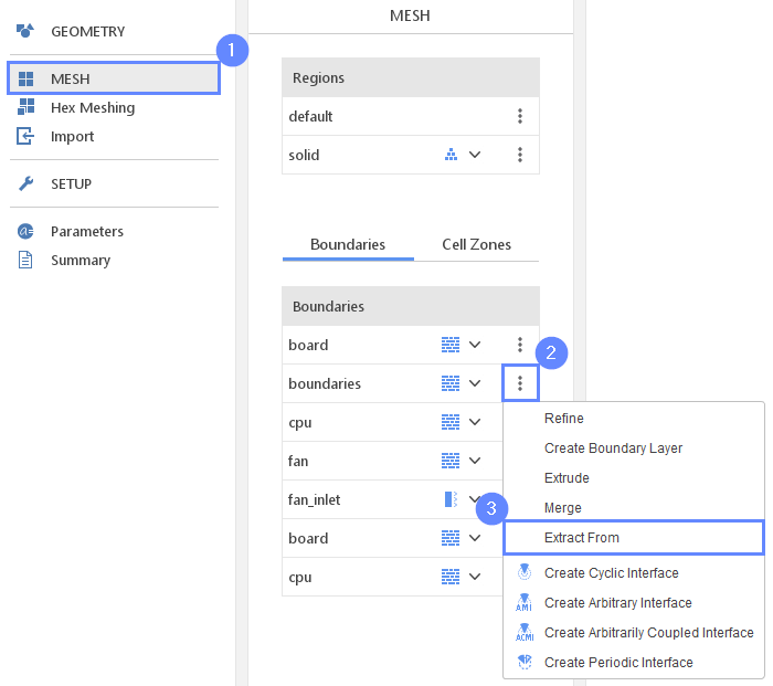
23. Fluid Mesh - Extract Outlet (I)
In the geometry setup, you created outlet_tool . You will now use this box to extract patch from boundary patch
- Go to MESH panel
- Click Options button next to boundaries patch
- Select Extract From option
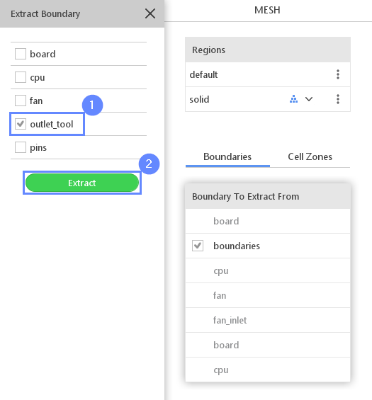
24. Fluid Mesh - Extract Outlet (II)
- Pick outlet_tool from the list
- Click Extract
The new patch will appear on the list of boundaries
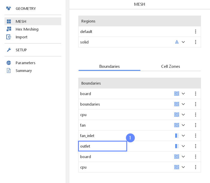
25. Fluid Mesh - Outlet
Now we have to rename the newly created boundary
- Change the boundary name
boundaries_in_outlet_tool \(\rightarrow\) outlet
26. Fluid Mesh - Create Sub-region
Now, after you used the Extract tool on the default mesh, you can convert it into a sub-region. It’s important to note that extract operations are no longer available once the mesh is converted.
- Expand the Options list next to the default region
- Select Make sub-region
- Enter Region Name to fluid
- Press OK
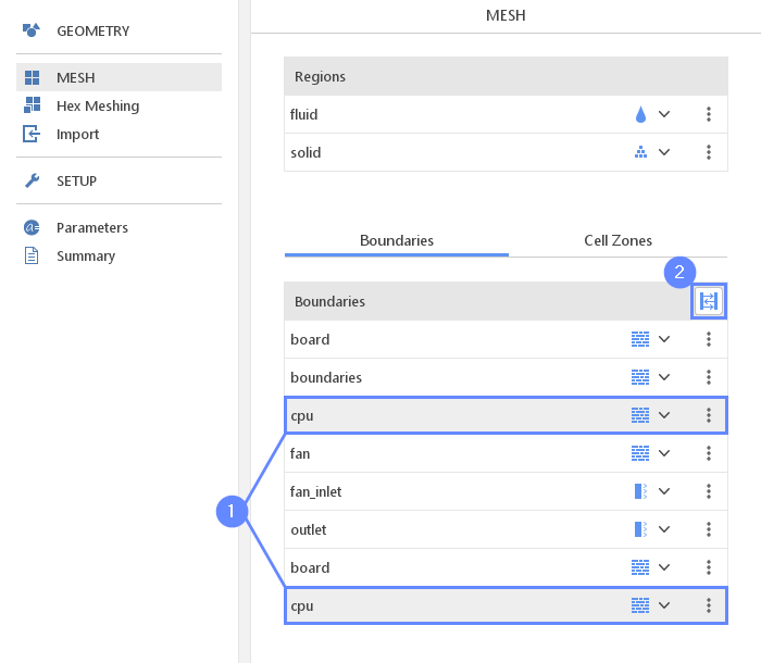
27. Create Region Interface
Two mesh regions are not coupled until you create a region interface. It will be further used to define which information is exchanged between regions.
- Select the cpu in fluid region and the cpu in solid region
(hold CTRL key and select both boundaries) - Press Create Region Interface
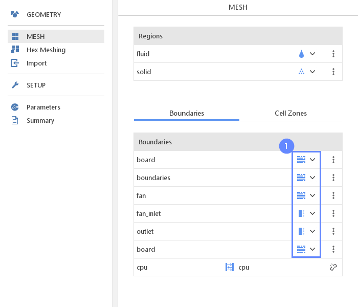
28. Set Boundary Conditions
- Make sure the boundary conditions are as follows
board wall
boundaries wall
fan wall
fan_inlet patch
outlet patch
board wall
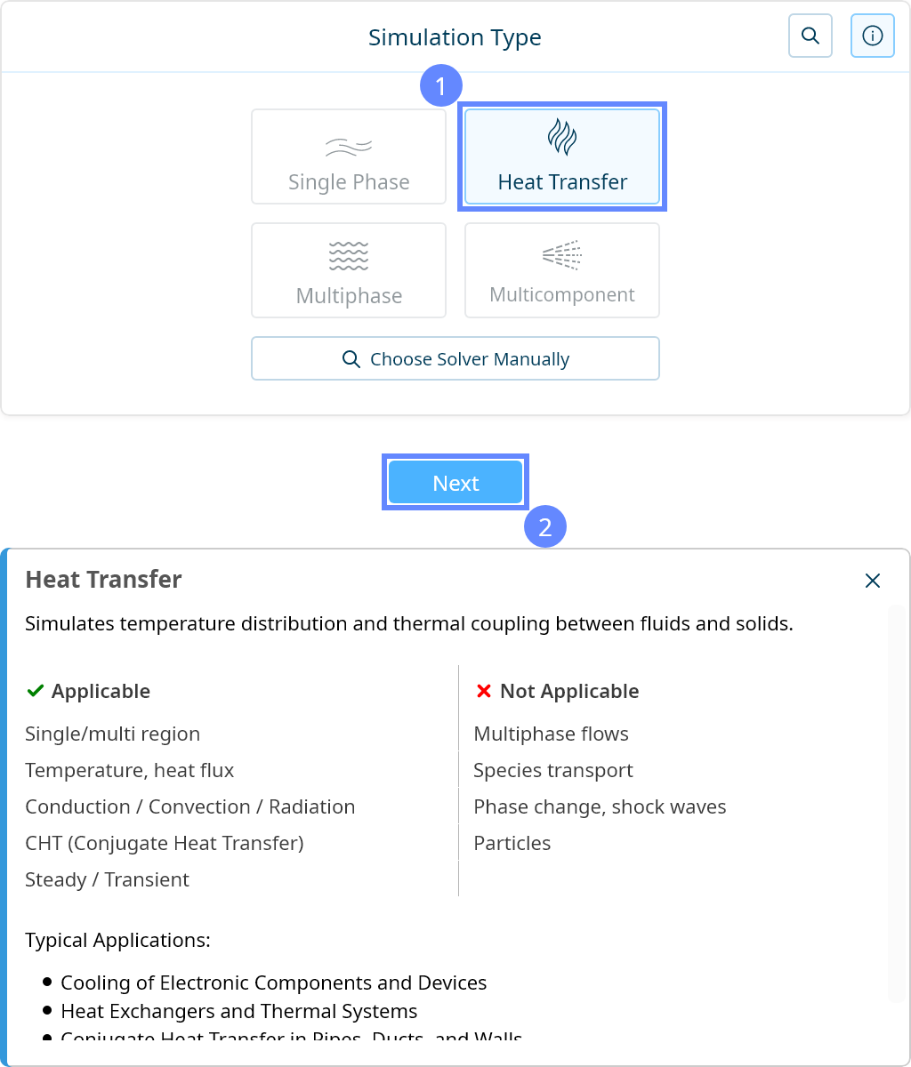
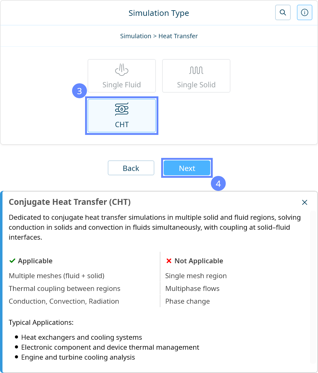
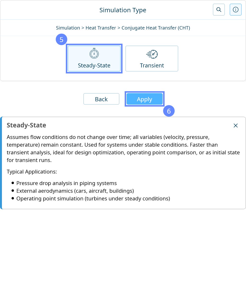
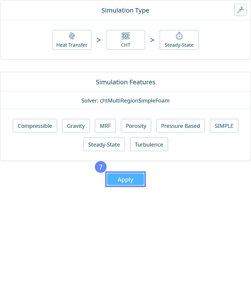
29. Simulation Type
We want to analyze the cooling of electronic components. For this purpose, we will use a steady-state conjugate heat transfer simulation with radiation modeling.

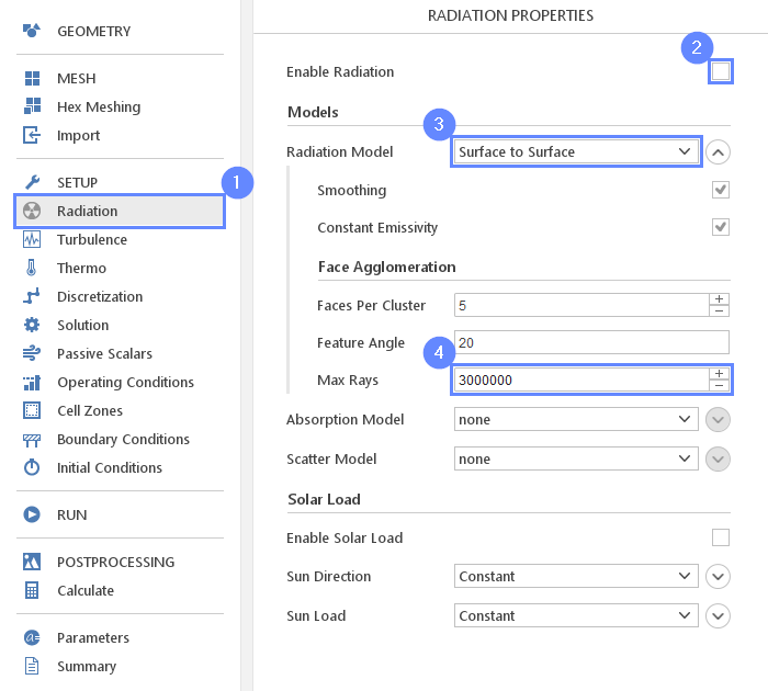
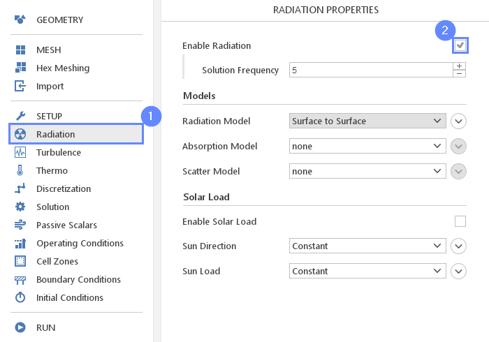
30. Radiation
We will first run a simulation without taking radiative heat transfer into account. However, it is important to set up all radiation model parameters now (these parameters cannot be changed later without resetting simulation).
- Go to Radiation panel
- Uncheck Enable Radiation
- Set Radiation Model to Surface To Surface
- Increase the Max Rays number to 3000000
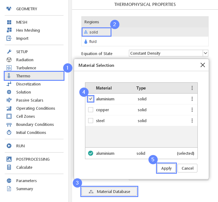
31. Thermophysical Properties of Solid
Now we need to define solid and fluid properties. We will assume that the working fluid is air and the solid is made of aluminum.
- Go to Thermo panel
- Select solid region
- Click Material Database button
- Select aluminium material
- Click Apply
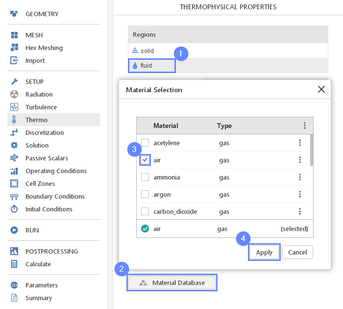
32. Thermophysical Properties of Fluid (I)
- Select fluid region
- Click Material Database button
- Select air material
- Click Apply
33. Thermophysical Properties of Fluid (II)
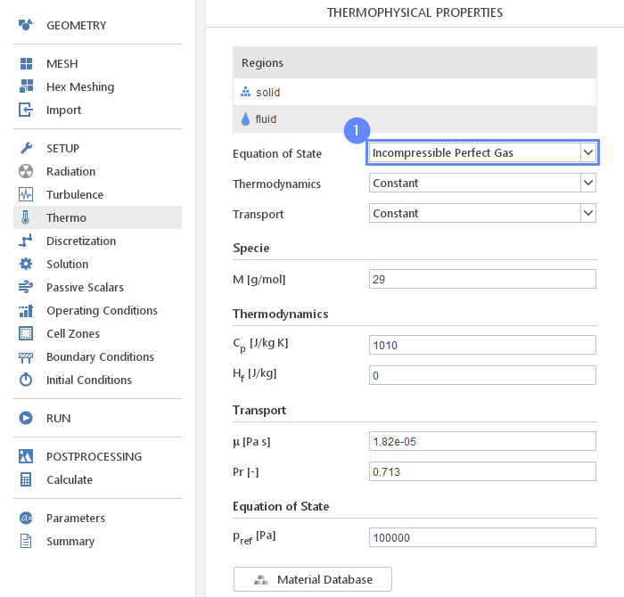
- Set the Equation of State to Incompressible Perfect Gas
34. Turbulence
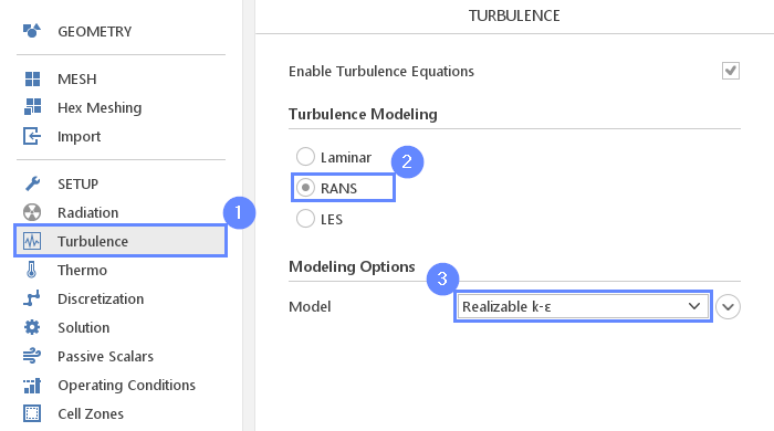
For turbulence modeling, we will use \(Realizable \; k{-} \varepsilon\) model
- Go to Turbulence panel
- Select RANS turbulence formulation
- Select \(Realizable \; k{-} \varepsilon\) model
35. Solution - Solvers
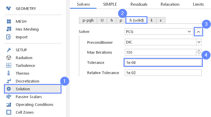
We will now adjust the solver tolerance threshold of the enthalpy equation in the solid region in order to achieve better convergence
- Go to Solution panel
- Select h (solid) tab
- Expand solver options
- Lower solver Tolerance to 1e-08
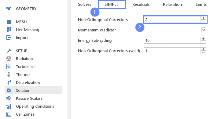
36. Solution - SIMPLE
To achieve better convergence we will adjust SIMPLE algorithm settings.
- Go to the SIMPLE tab
- Increase number of Non-Orthogonal Correctors to 2
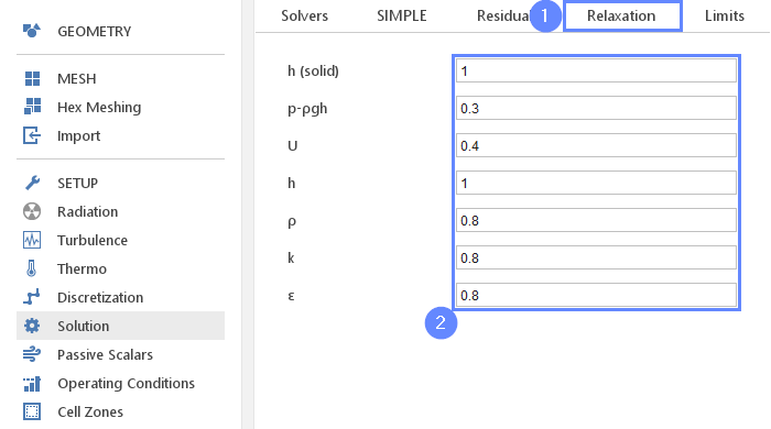
37. Solution - Relaxation
- Go to Relaxation tab
- Adjust relaxation coefficients
\(h(solid)\)1
\(p {-} \rho gh\)0.3
\(U\)0.4
\(h\)1
\(\rho\)0.8
\(k\)0.8
\(\varepsilon\)0.8
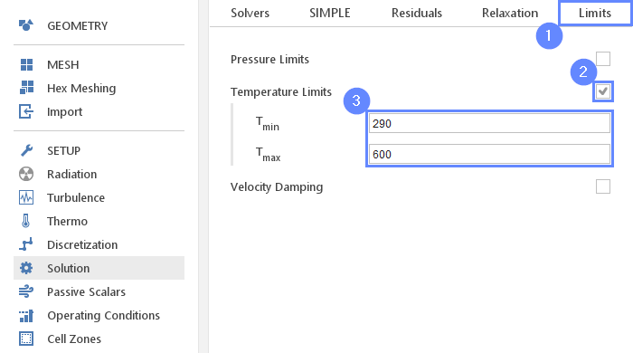
38. Solution - Limits
Now, we will adjust the limits of temperature fields in order to narrow the convergence space of the solution
- Go to Limits tab
- Enable Temperature Limits
- Adjust minimum and maximum temperature to a reasonable range
\(T_{min}\)290
\(T_{max}\)600
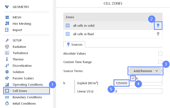
39. Cell Zones
Now set heat source term in the CPU volume. In this tutorial, we assume that only the CPU produces the heat of power of 0.25 W and its volume is about 200 mm 3 :
- Go to Cell Zones setup
- Enable Source term for all cells in solid
- Click Add/Remove in Source Terms
- Select h equation
- Set explicit source term
h Explicit \({\sf [W/m^3]}\)1250000
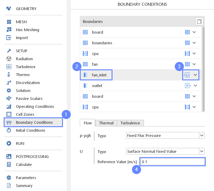
40. Boundary Conditions - Inlet (Flow)
Now, we will define the inlets and outlet boundary conditions. On the inlet, we will set constant air inflow.
- Go to Boundary Conditions panel
- Select fan_inlet boundary
- Set the Velocity Inlet character
- Set the inlet velocity
U Reference Value \({\sf [m/s]}\)0.1
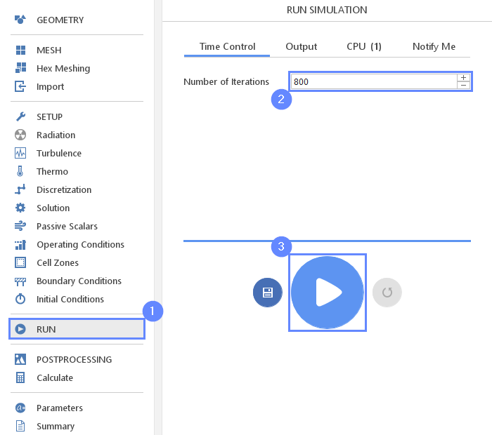
41. Run - Time Control
- Go to Run panel
- Set Number of Iterations to 800
- Click Run Simulation button
Estimated computation time: 10 minutes
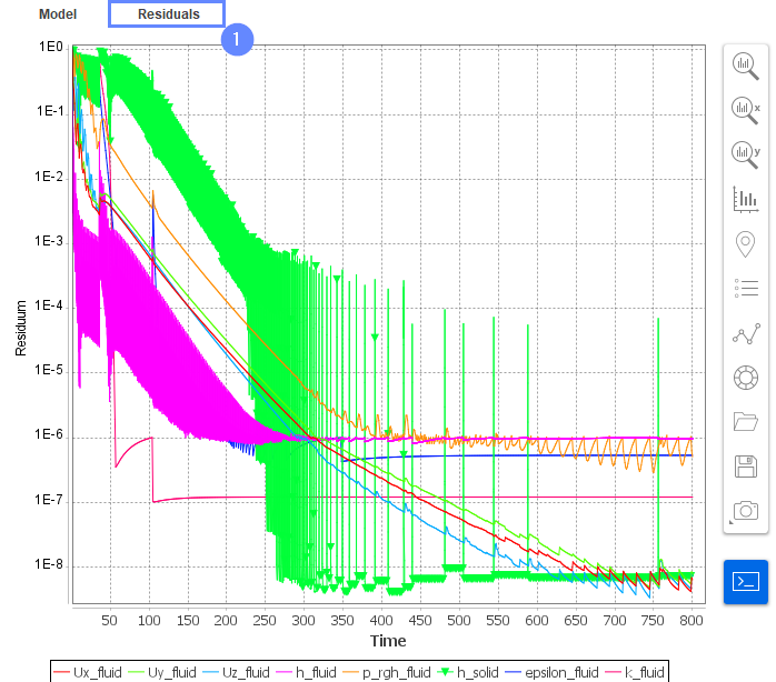
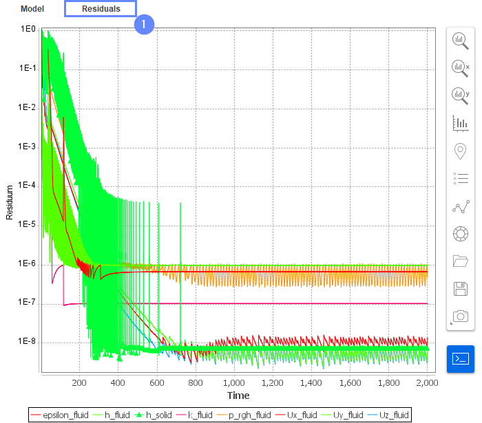
42. Residuals
- Monitor convergence process under Residuals tab
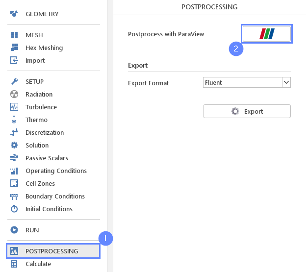
43. Start Postprocessing - ParaView
Start ParaView software to display results
- Go to Postprocessing panel
- Start ParaView
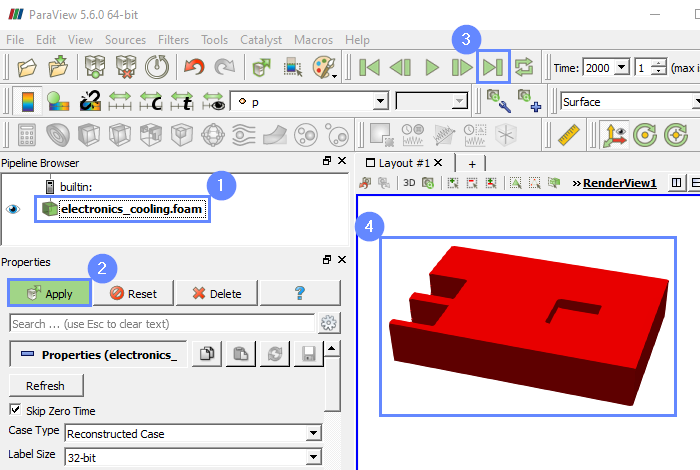
44. ParaView - Load Results
- Select electronics_cooling.foam
- Click Apply to load results
- Click Last Frame to select the latest result set
- After loading results they will be shown in the 3D graphic window

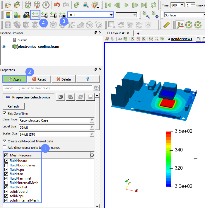
45. ParaView - Display Temperature Contour (I)
We will now plot the temperature contour on the circuit board again. We will use the same scale, so the differences in results are more evident
- Select the following mesh regions
/fluid/patch/board
/fluid/patch/cpu
/fluid/patch/fan
/fluid/patch/fan_inlet
/fluid/patch/outlet
/solid/patch/board
/solid/patch/cpu
/solid/internalMesh
(you can check Mesh Regions to select all regions and uncheck others: /fluid/group/viewFactorWall, /fluid/patch/boundaries and /fluid/internalMesh ) - Click Apply
- Select contour coloring variable to T
- Click Rescale to Data Range
46. ParaView - Display Temperature Contour (II)
Results are displayed in the graphics window. Note that the maximum temperature in the domain is about 355 K.
47. Radiation Setup
We will now enable the radiation equation in our simulation. To do this, close Paraview and go back to SimFlow
- Go to Radiation panel
- Check Enable Radiation
48. Start Simulation with Radiation
The case is set up. We will increase the number of iterations and run the simulation
- Go to Run panel
- Set Number of Iterations to 2000
- Click Continue Simulation button
Estimated computation time: 20 minutes

49. Residuals (II)
- Monitor convergence process under Residuals tab
50. ParaView - Start Postprocessing (with Radiation)
Start ParaView software to display results
- Go to Postprocessing panel
- Start ParaView

51. ParaView - Load Results (with Radiation)
- Select electronics_cooling.foam
- Click Apply to load results
- Click Last Frame to select the latest result set
- After loading results they will be shown in the 3D graphic window
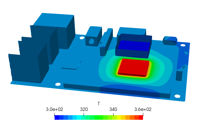
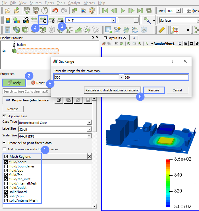
52. ParaView - Display Temperature Contour (with Radiation) (I)
You will now plot the temperature contour on the circuit board again. You will use the same scale, so the differences in results are more evident
- Select the followings mesh regions
/fluid/patch/board
/fluid/patch/cpu
/fluid/patch/fan
/fluid/patch/fan_inlet
/fluid/patch/outlet
/solid/patch/board
/solid/patch/cpu
/solid/internalMesh
(you can check Mesh Regions to select all regions and uncheck others: /fluid/group/viewFactorWall, /fluid/patch/boundaries and /fluid/internalMesh ) - Click Apply
- Select contour coloring variable to T
- Select Rescale to Custom Data Range
- Set minimum and maximum value
Min 300 Max 360 - Click Rescale
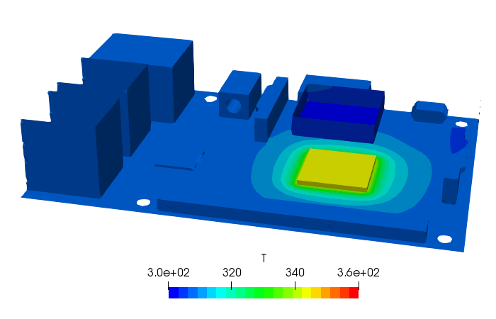
53. ParaView - Display Temperature Contour (with Radiation) (II)
Results are displayed in the graphics window. Note that in this case, the maximum temperature in the domain is 340 K, which is 17 K lower than in the previous simulation.
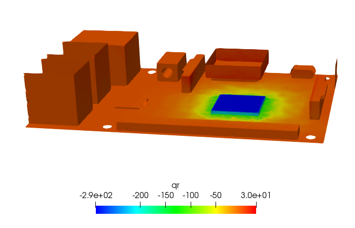
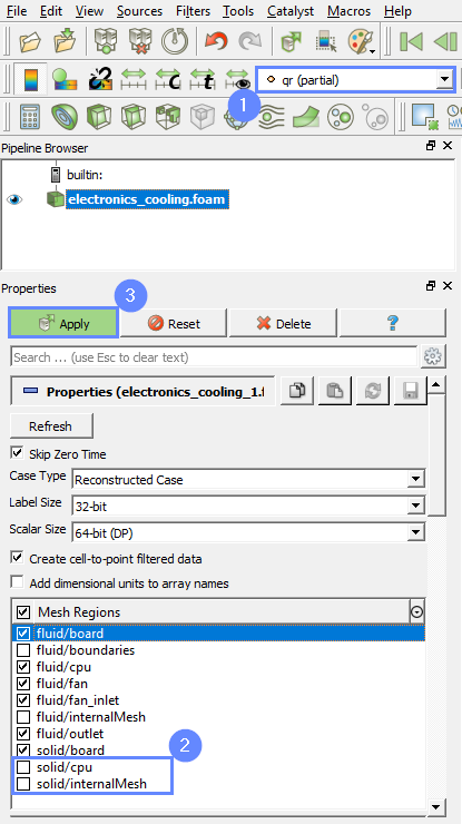
54. ParaView - Radiative Heat Flux (I)
Radiation plays an important role in this scenario. Therefore, our last task will be to display radiative heat flux mapped on the geometry
- Set contour coloring variable to qr(partial)
- Uncheck mesh regions solid/rPi2_CPU and solid/internalMesh
- Click Apply
55. ParaView - Radiative Heat Flux (II)
Results are displayed in the graphics window.
| Note that this tutorial is meant only to demonstrate the capabilities of the software and not to solve the problem in the best possible way. Therefore, some assumptions are taken to keep case setup time and computational time low. In particular, to refine the model, one could in first place consider setting more suitable emissivity coefficients for materials used. |