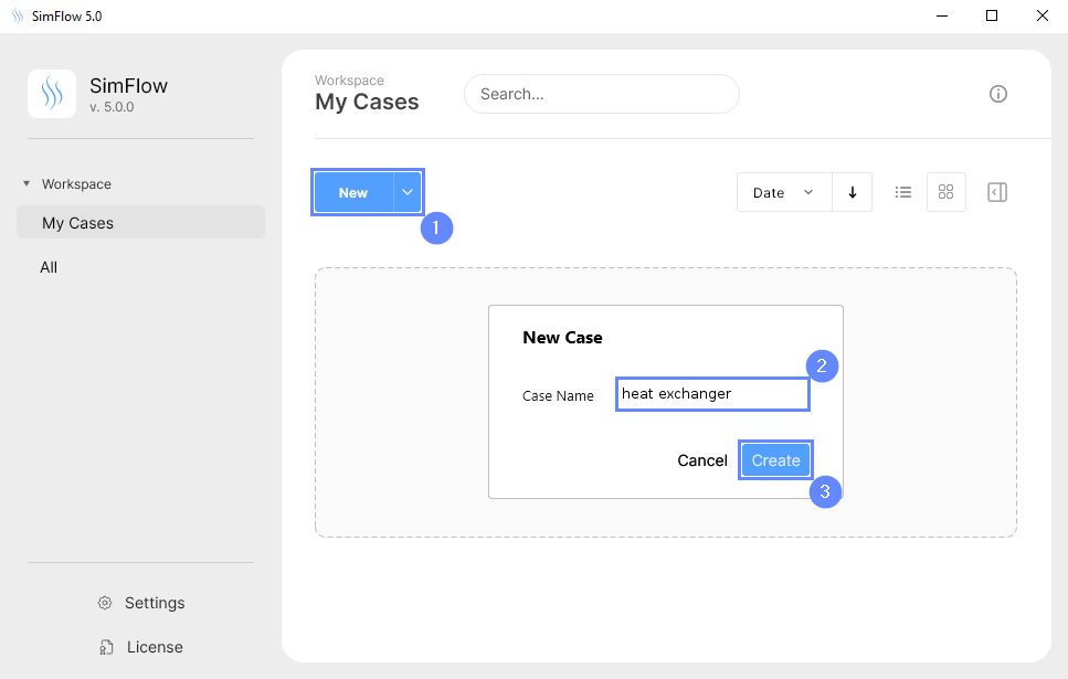
3. Create Case
Open SimFlow and create a new case named heat exchanger
- Click New
- Provide name heat exchanger
- Click Create to open a new case button
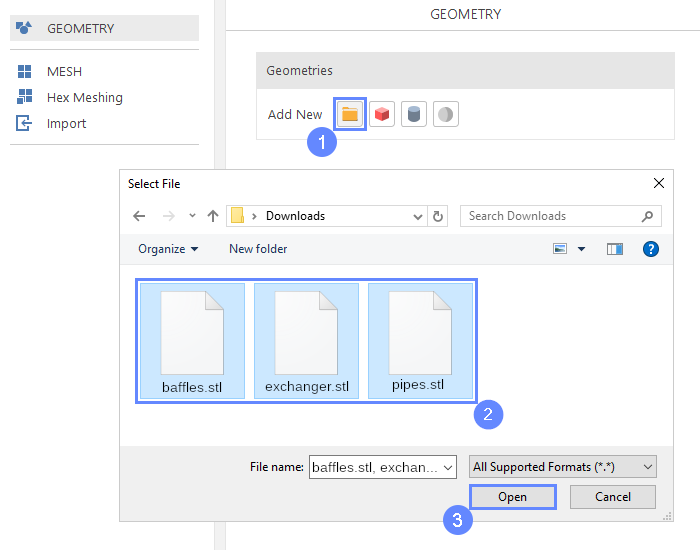
4. Import Geometry - Heat Exchanger
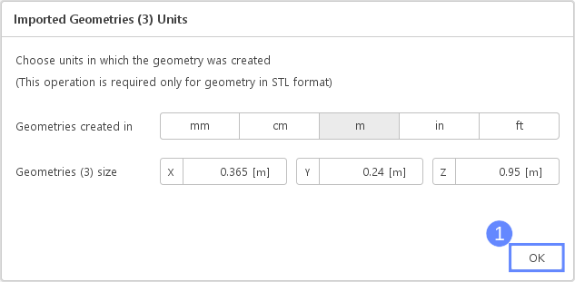
5. Imported Geometry Units
The STL format does not contain the unit information which are defined during the geometry export. Therefore, you must manually specify the correct unit after import. If we do not know the exported unit, we can estimate it based on the total size of imported geometries. The size is displayed next to Geometry size label. In our case, the default unit meter is correct.
- To confirm default unit meter, press OK
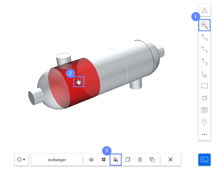
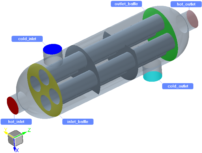
6. Geometry - Heat Exchanger
After importing geometry, it will appear in the 3D window. We will make the exchanger geometry transparent to see the interior of the heat exchanger.
- Click Fit View to zoom the geometry
- Hold the CTRL key and click exchanger wall
- Select Display Properties
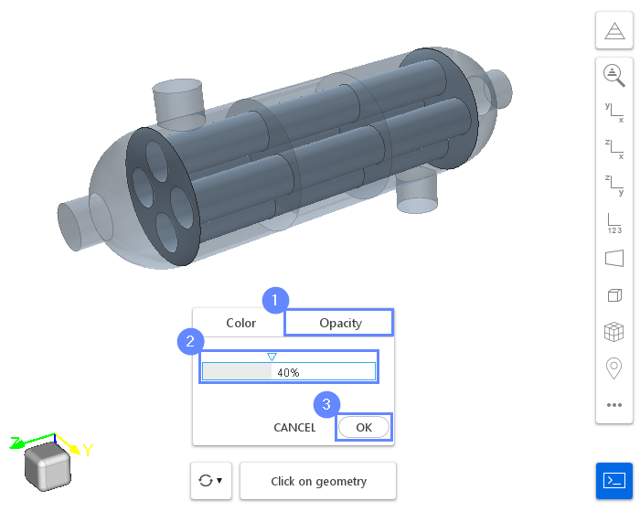
7. Change Opacity - Heat Exchanger
- Select Opacity tab
- Adjust opacity to 40%
- Click OK to apply
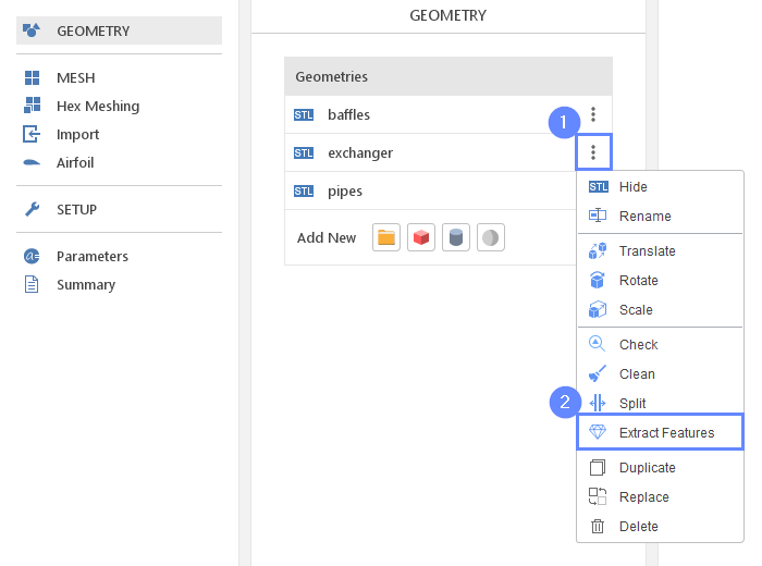
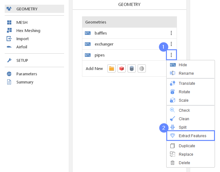
8. Extract Geometry – Exchanger(I)
To reveal edges, we will use Extract Features operation. These edges will indicate additional mesh refinement regions.
- Extend Options list next to the exchanger geometry
- Select Extract Features
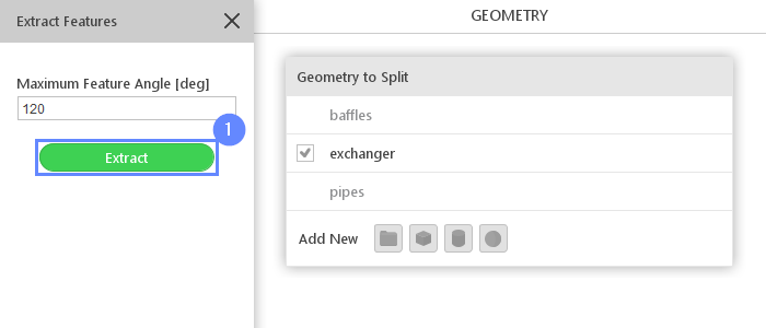
9. Extract Geometry – Exchanger(II)
- Select Extract
10. Extract Geometry – Pipes (I)
Repeat extract operation for the pipes
- Extend Options list next to the pipes geometry
- Select Extract Features
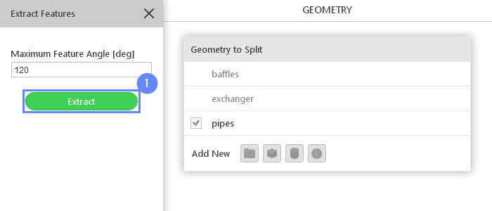
11. Extract Geometry – Pipes (II)
- Select Extract
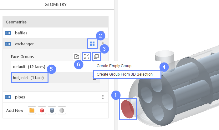
12. Create Face Groups (I)
We need to distinguish surfaces that will be used as the mesh boundaries (both external and internal). We will do it in the 3D graphical panel.
- Select first inlet face
(hold Ctrl and left-click on the geometry face) - Click Geometry Faces next to exchanger
- Click Create New Face Group
- Click Create Group From 3D Selection
- Rename group_1 to hot_inlet
(double click on the group to rename, press Enter to confirm) - Click Clear Selection to deselect faces
(use before creating new selection within the same geometry)
13. Create Face Groups (II)
We will repeat the previous operations for the remaining inlets and outlets. The final face groups list for exchanger should look like below:
- hot_inlet (darak red)
- hot_outlet (light red)
- cold_inlet (dark blue)
- cold_outlet (light blue)
To create face groups for pipes geometry, hide the exchanger geometry first. Then create two face groups like below: - inlet_baffle (yellow)
- outlet_baffle (green)
| Tip #1 To select a single face, first exit selection by clicking Esc |
| Tip #2 To hide exchanger geometry, click the STL icon to the left of its name |
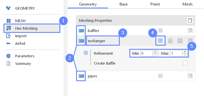
15. Hot Fluid Mesh - Meshing Parameter - Exchanger
Hot fluid region
We will start meshing from the hot fluid region.
- Go to Hex Meshing panel
- Make sure that all geometries are visible
(you can unhide the geometry by clicking the icon next to the geometry name) - Select exchanger geometry
- Enable Mesh Geometry
- Set Refinement to Min 0 Max 1
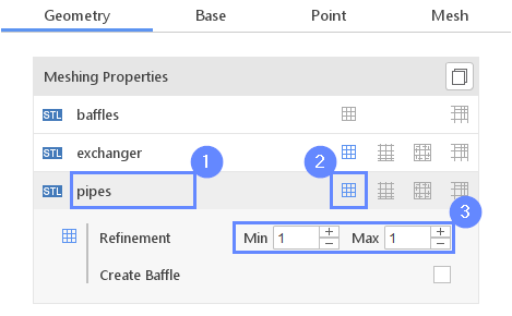
16. Hot Fluid Mesh - Meshing Parameter - Pipes
- Select pipes geometry
- Enable Mesh Geometry
- Set Refinement to Min 1 Max 1
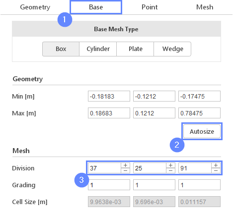
17. Base Mesh
We need to define the base mesh. The box geometry determines the background mesh domain. It encloses both fluid regions – hot and cold.
- Go to Base tab
- Press Autosize button
(make sure that all geometries are visible – autosize option adjust the base mesh only to the visible geometry) - Define the number of divisions
Division372591
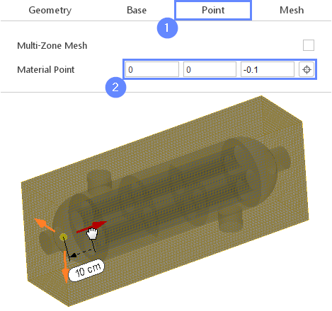
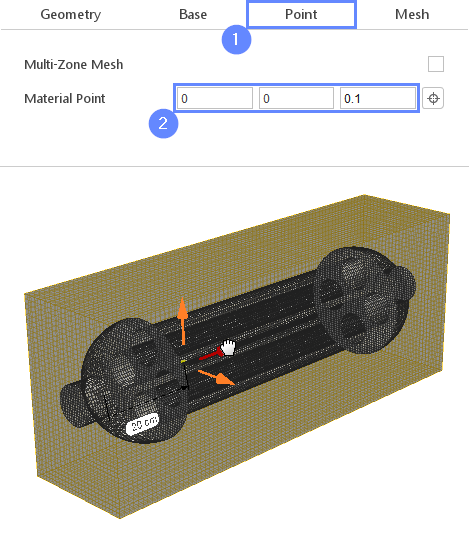
18. Hot Fluid Mesh - Material Point
In order to create the mesh in the hot fluid region, we will place the material point inside the hot fluid sub-domain. The resulting mesh will remain only in this region.
- Go to Point tab
- Specify location inside the hot fluid region
Material Point00-0.1
You can specify the point location from the 3D view. Hold the Ctrl key and drag the arrows to the destination.
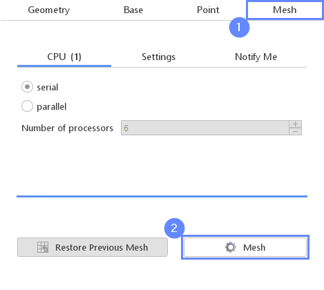
19. Hot Fluid Mesh - Start Meshing
Now, it’s time to create the mesh of the hot fluid region.
- Go to Mesh tab
- Start the meshing process with Mesh button

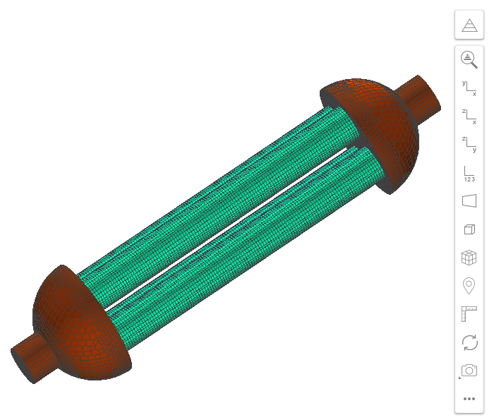
20. Hot Fluid Mesh
When the meshing process is finished, the hot fluid region mesh appears on the screen.
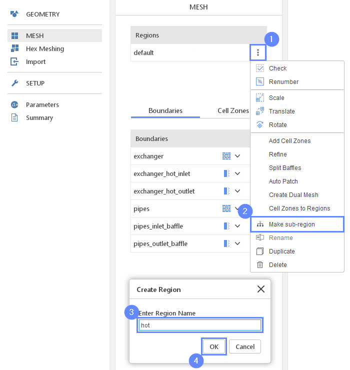
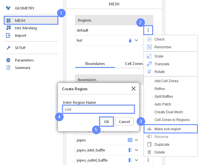
21. Hot Fluid Mesh - Create Sub-region
For the CHT simulations, we need to mark each of the mesh regions as sub-domains. The sub-domains represent a partial mesh that will not be overwritten by meshing operations that use the default region as a target.
- Expand the Options list next to the default region
- Select Make sub-region
- Enter Region Name to hot
- Press OK
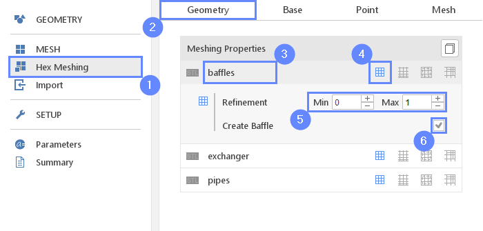
22. Cold Fluid Mesh - Meshing Parameter - Baffles
Cold fluid region
Now we can mesh the second region – the cold fluid region. We will use already defined geometry parameters for exchanger and pipes. We just need to add baffles to be included in the mesh.
- Go to the Hex Meshing panel
- Go to the Geometry tab
- Select baffles
- Enable Mesh Geometry
- Set Refinement to Min 0 Max 1
- Turn on Create Baffle
23. Cold Fluid Mesh - Material Point
We need to move the material point to be positioned inside the cold fluid region.
- Go to Point tab
- Specify location inside the hot fluid region
Material Point000.1
24. Cold Fluid Mesh - Start Meshing
Now, it’s time to create the mesh of the cold fluid region. Please note that the resulting mesh will be automatically assigned to the default region and will exist next to the previously created hot fluid mesh.
- Go to Mesh tab
- Start the meshing process with Mesh button
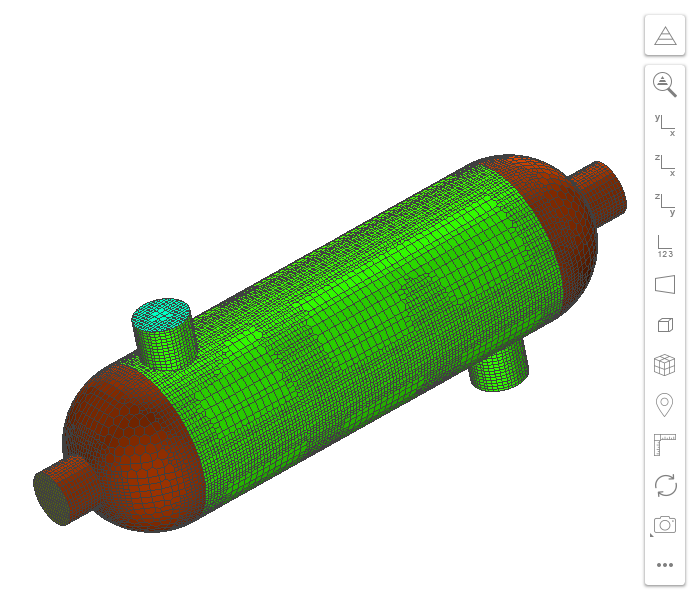
25. Mesh
The complete mesh should look like in the picture below.
26. Cold Fluid Mesh - Create Sub-region
Move the default region into the cold fluid region. The CHT simulation can only use the sub-region meshes.
- Go to MESH panel
- Expand the Options list next to the default region
- Select Make sub-region
- Enter Region Name to cold
- Press OK
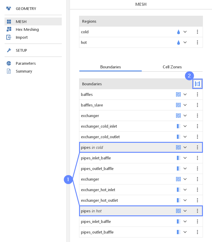
27. Create Mesh Interface (I)
In the previous steps we have created the mesh for hot and cold fluid regions. At the moment they are treated separately, so the information on the flow cannot be exchanged between them. It’s time to create the interface (coupling) between both fluid regions. Later, we will define boundary conditions which will describe the way we want to exchange information between hot and cold fluid region.
- Select the pipes in cold fluid region and the pipes in hot fluid region
(hold CTRL key and select both boundaries) - Press Create Region Interface
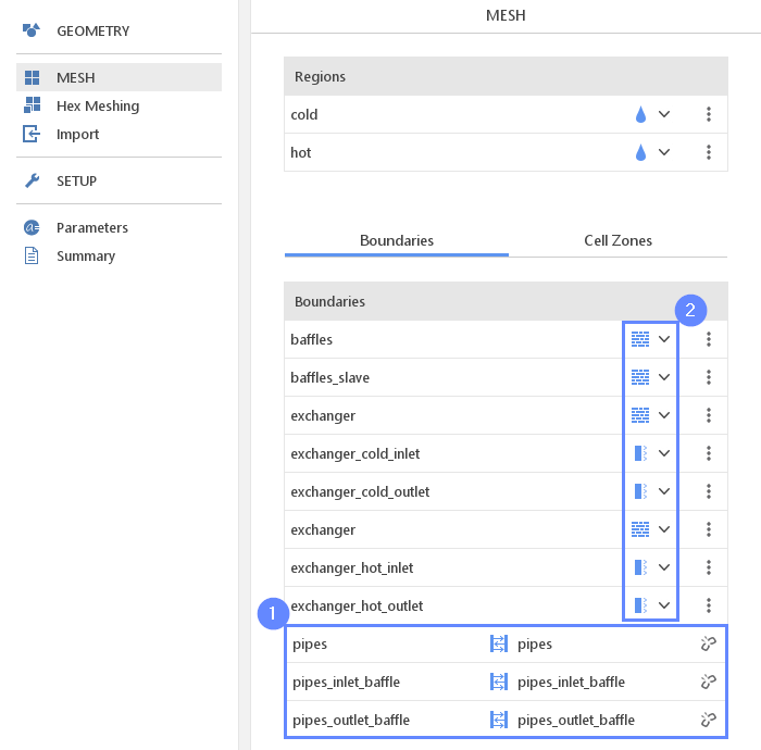
28. Create Mesh Interface (II)
- Repeat previous steps for pipes_inlet_baffle and pipes_outlet_baffle couple. Check the interfaces list
pipes in cold \(\leftrightarrow\) pipes in hot
pipes_inlet_baffle in cold \(\leftrightarrow\) pipes_inlet_baffle in hot
pipes_outlet_baffle in cold \(\leftrightarrow\) pipes_outlet_baffle in hot - Adjust the remaining boundaries types
baffles wall
baffles_slave wall
exchanger _in cold _wall
exchanger_cold_inlet patch
exchanger_cold_outlet patch
exchanger _in hot _wall
exchanger_hot_inlet patch
exchanger_hot_outlet patch
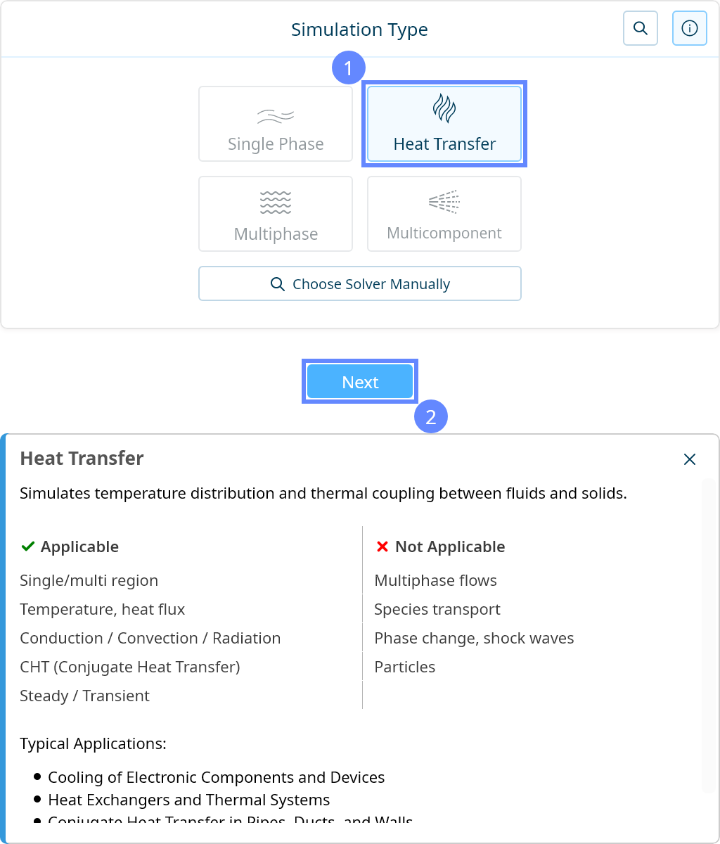
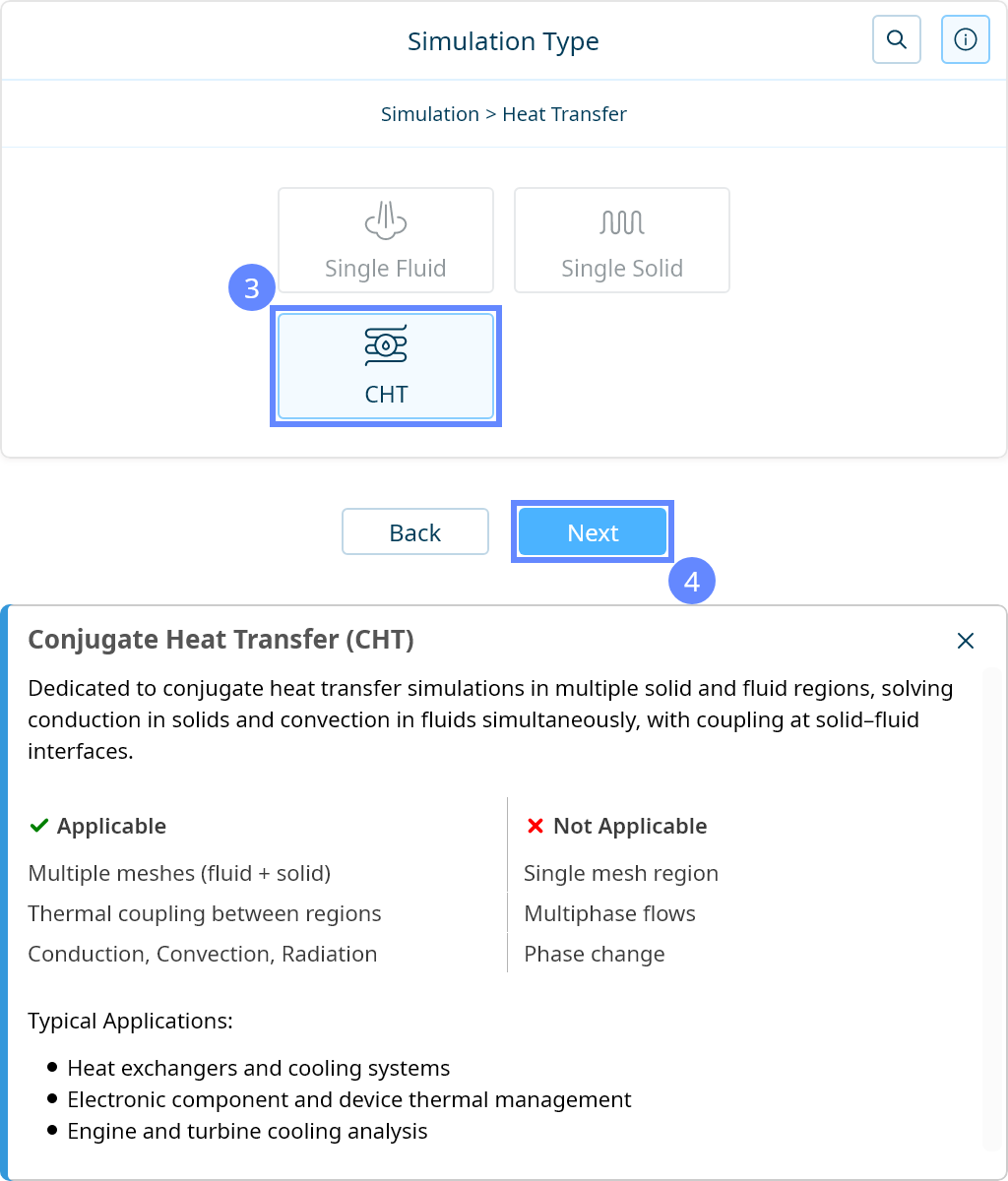
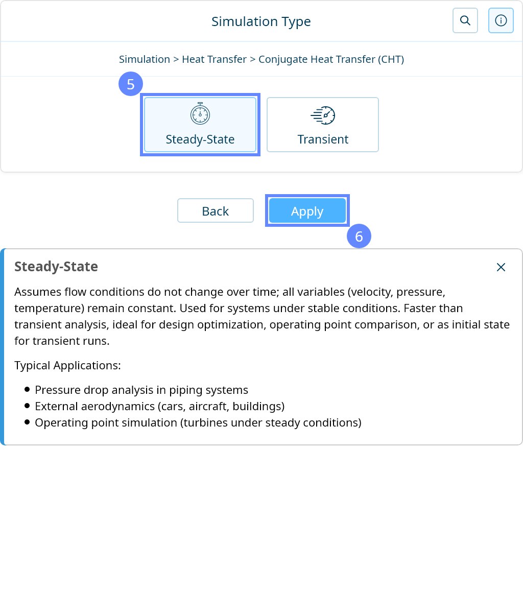
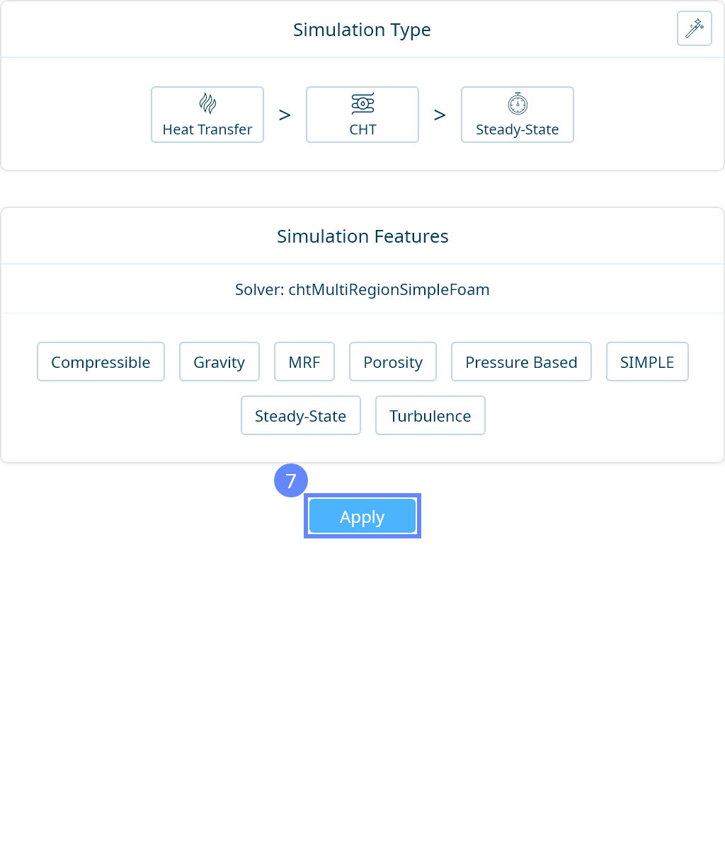
29. Simulation Type
We want to analyze heat transfer efficiency in a heat exchanger. For this purpose, we will use a steady-state conjugate heat transfer simulation.

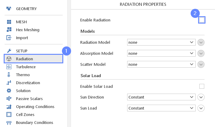
30. Radiation
We will disable radiation for our simulation.
- Go to Radiation panel
- Uncheck Enable Radiation option
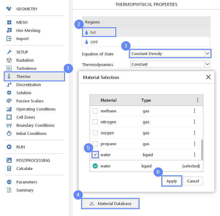
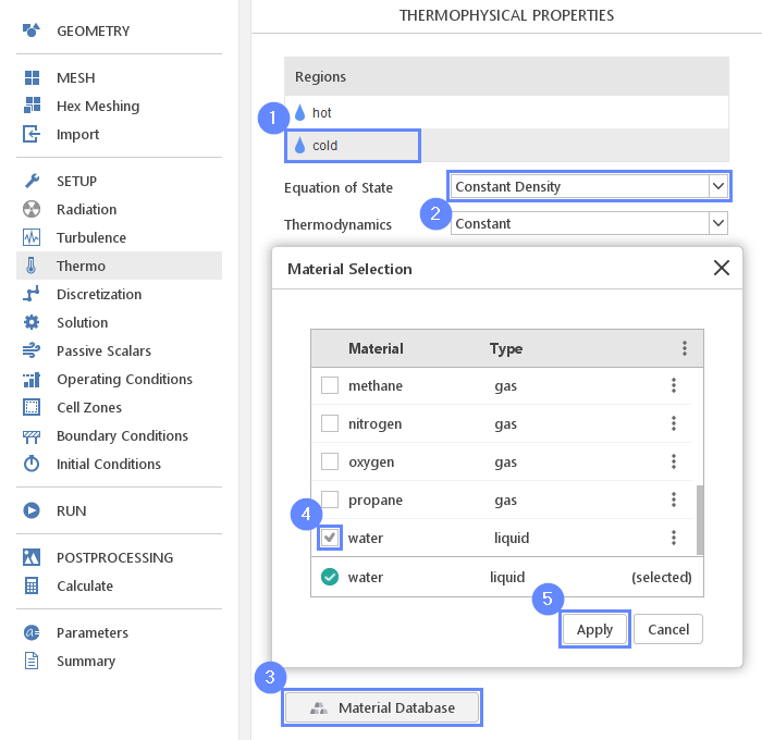
31. Thermo - Fluid Properties - Hot Region
Now we need to define fluid properties. We will assume that working fluid for hot and cold regions is water.
- Go to Thermo panel
- Select hot region
- Select Constant Density for Equation of State
- Open Material Database
- Scroll down to find water
- Click Apply
32. Thermo - Fluid Properties - Cold Region
- Select cold region
- Select Constant Density for Equation of State
- Open Material Database
- Scroll down to find Water
- Click Apply
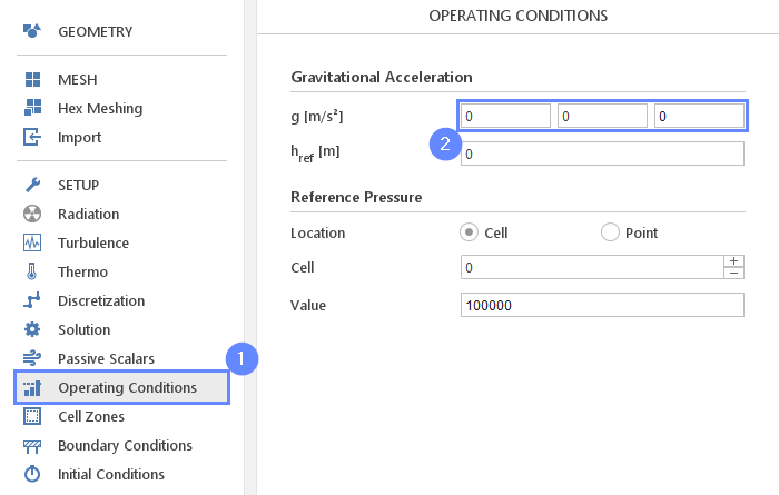
33. Operating Conditions
We will turn off the gravity acceleration.
- Go to Operating Conditions panel
- Set non Gravity Acceleration
g \({\sf [m/s^2]}\)000
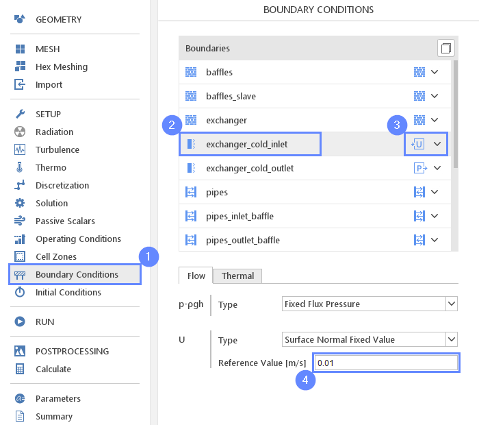
34. Boundary Conditions - Exchanger Cold Inlet - Flow
We will leave the default conditions for the baffles and heat exchanger external surfaces – adiabatic (isolated) walls. Now, we will define the inlets and outlets parameters for hot and cold regions.
- Go to Boundary Conditions panel
- Select exchanger_cold_inlet boundary
- Set the Velocity Inlet character
- Set the inlet velocity
U Reference Value \({\sf [m/s]}\)0.01
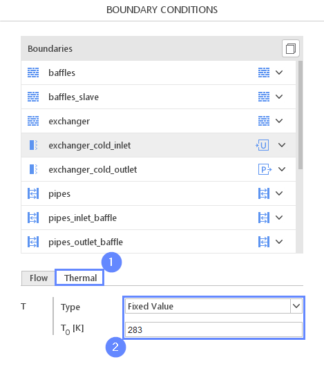
35. Boundary Conditions - Exchanger Cold Inlet - Thermal
- Go to Thermal tab
- Set the type and value
T Type Fixed Value
T \(T_0\) \({\sf [K]}\)283
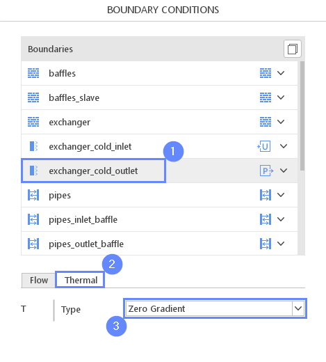
36. Boundary Conditions - Exchanger Cold Outlet
- Select exchanger_cold_outlet
- Switch to Thermal tab
- Set the Type to Zero Gradient
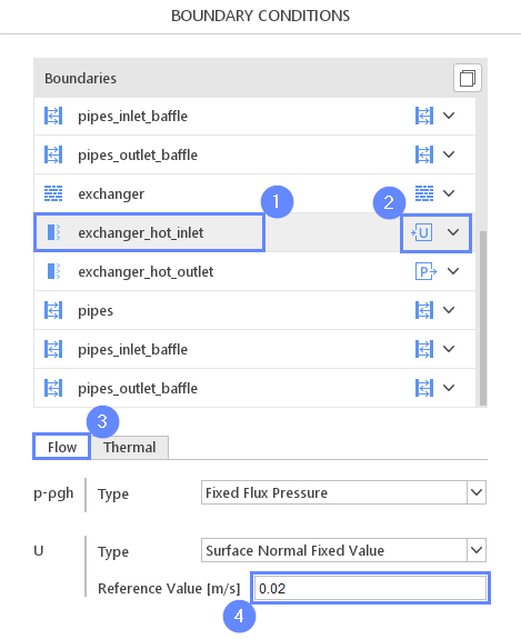
37. Boundary Conditions - Exchanger Hot Inlet - Flow
- Select exchanger_hot_inlet boundary
- Set the Velocity Inlet character
- Switch to Flow tab
- Set the inlet velocity
U Reference Value \({\sf [m/s]}\)0.02
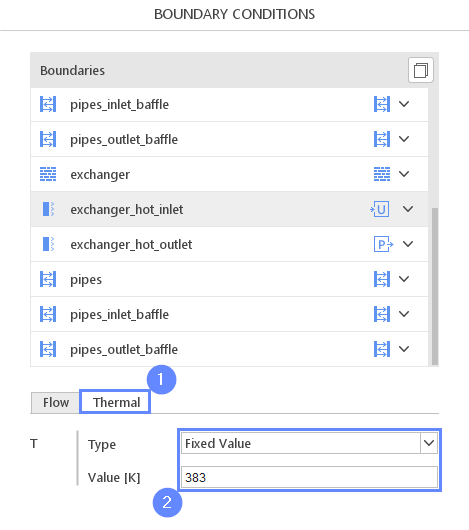
38. Boundary Conditions - Exchanger Hot Inlet - Thermal
- Go to Thermal tab
- Set the type and value
T Type Fixed Value
T \(T_0\) \({\sf [K]}\)383
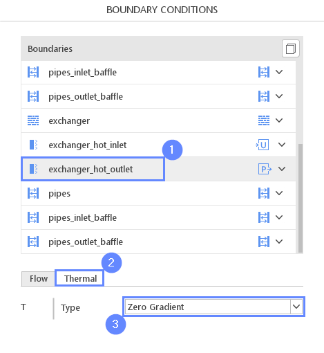
39. Boundary Conditions - Exchanger Hot Outlet
- Select exchanger_hot_outlet
- Switch to Thermal tab
- Set the Type to Zero Gradient
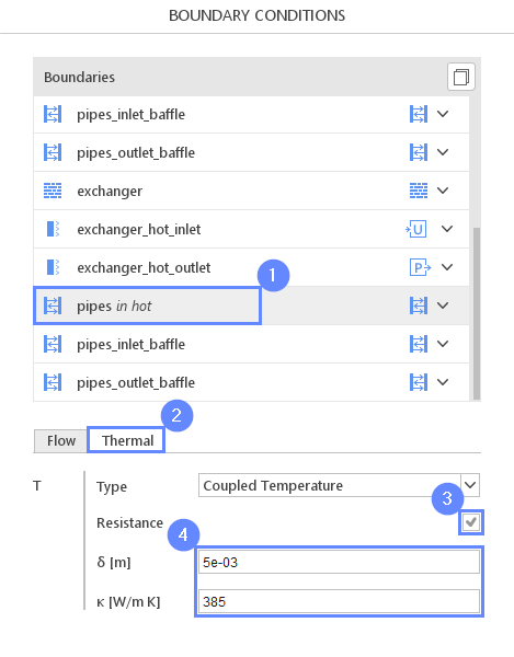
41. Boundary Conditions - Pipes - Thermal
We will apply the same settings for other interfaces under hot region: pipe , pipes_inlet_baffle and pipes_outlet_baffle boundaries.
- Select pipes (hot region)
- Go to Thermal tab
- Check the Resistance
- Set the thickness of the wall and thermal conductivity
T \(\sigma\) \({\sf [m]}\)5e-03
T \(\kappa\) \({\sf [W/m \cdot K]}\)385
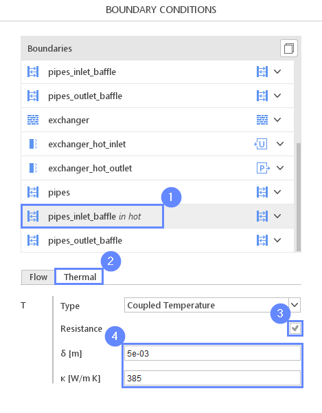
42. Boundary Conditions - Pipes Inlet Baffle - Thermal
- Select pipes_inlet_baffle (hot region)
- Go to Thermal tab
- Check the Resistance
- Set the thickness of the wall and thermal conductivity
T \(\sigma\) \({\sf [m]}\)5e-03
T \(\kappa\) \({\sf [W/m \cdot K]}\)385
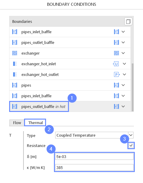
43. Boundary Conditions - Pipes Outlet Baffle - Thermal
- Select pipes_outlet_baffle (hot region)
- Go to Thermal tab
- Check the Resistance
- Set the thickness of the wall and thermal conductivity
T \(\sigma\) \({\sf [m]}\)5e-03
T \(\kappa\) \({\sf [W/m \cdot K]}\)385
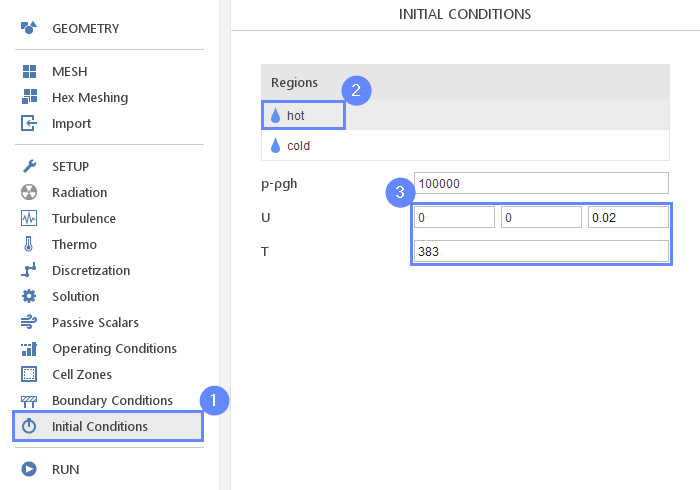
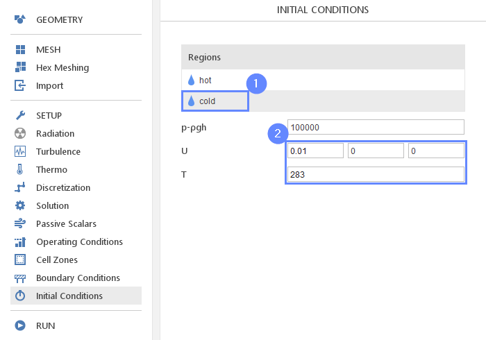
44. Initial Conditions - Hot Region
Before we start simulation, we need to define the initial conditions. We will adjust the initial velocity and temperature to the inlet conditions of each region.
- Go to Initial Conditions panel
- Select hot fluid region
- Define initial velocity and temperature
U000.02
T383
45. Initial Conditions - Cold Region
- Select cold fluid region
- Define initial velocity and temperature
U0.0100
T283
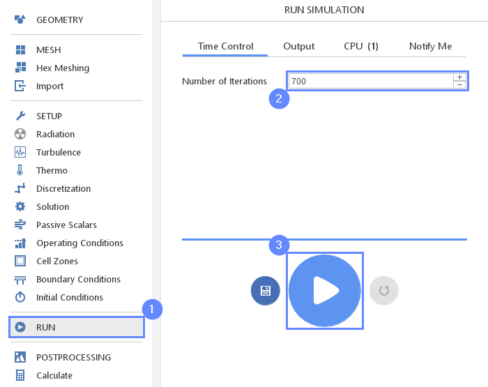
46. Run Simulation
Finally, we can start our computation.
- Go to Run panel
- Set Number of Iterations to 700
- Click Run Simulation
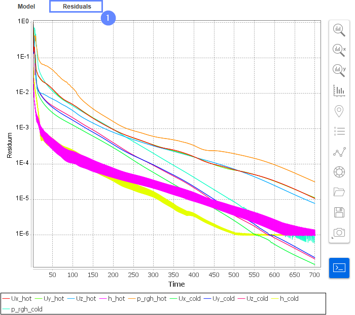
47. Residuals
- Monitor convergence process under Residuals tab
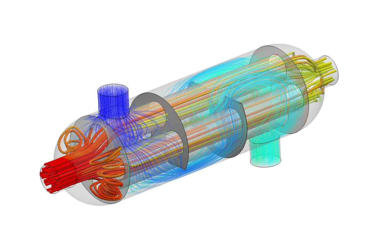
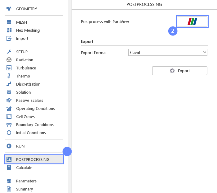
48. Postprocessing - ParaView
After computations are finished, we can do a complex visualization of our results with ParaView.
- Go to Postprocessing panel
- Click Run ParaView
If you do not plug in the new ParaView to SimFlow, you can just run the ParaView and open the case file:
` …/heat_exchanger/heat_exchanger/heat_exchanger.foam `
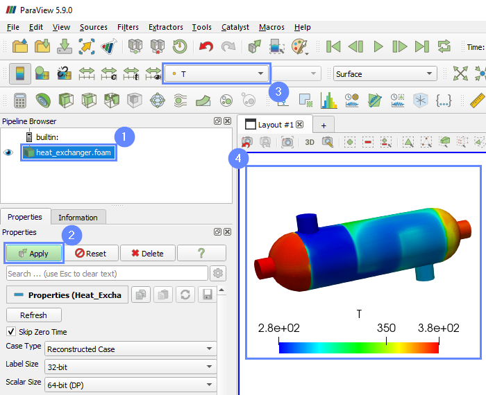
49. ParaView - Load Results
Load the results of the simulation from SimFlow
- Select heat_exchanger.foam
- Click Apply button to load results into ParaView
- Select Temperature from the drop-down list
- After loading results, they will be shown in the 3D graphic window
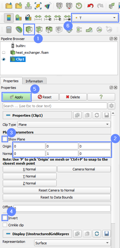
50. ParaView - Clip
We will create the cross-section through the computational domain to display the temperature distribution.
- Select Clip button
- Set the plane origin and normal
Origin000
Normal010 - Untick Show Plane
- Untick Invert
- Press Apply
- From the drop-down menu select Temperature
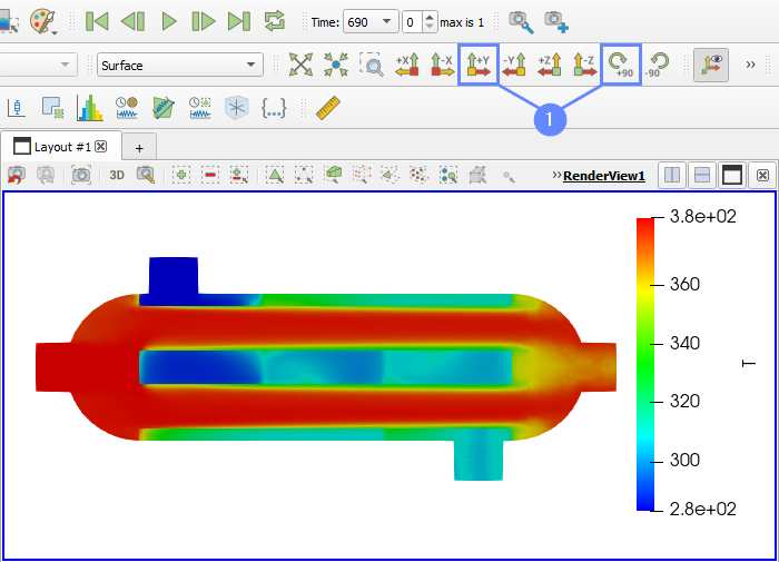
51. ParaView - Results
- Orient the view parallel the XZ plane and rotate 90 degrees clockwise