3. Create Case
This tutorial will require high CPU usage and might take several hours to finish the calculation depending on the machine used.
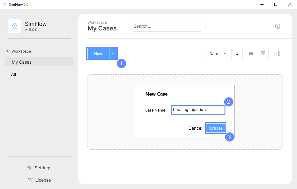
Open SimFlow and create a new case named housing injection
- Click New
- Provide name housing injection
- Click Create to open a new case
4. Import Geometry
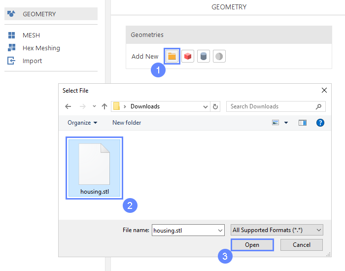
Firstly we need to Download GeometryHousing
- Click Import Geometry
- Select geometry file housing.stl
- Click Open
5. Imported Geometry Units
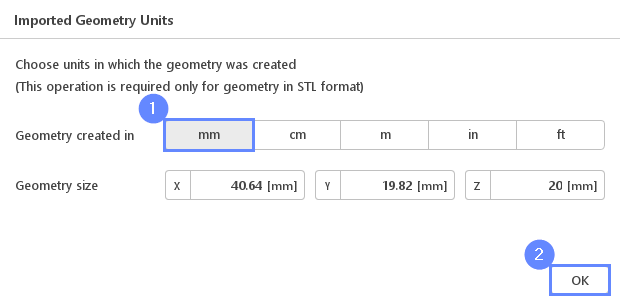
Since the imported geometry is in STL format, which does not store unit information, we need to confirm the unit in which the model was created. The Geometry size displays overall size of the model in each direction what should help to decide which unit is the valid one. In this case, the model was created in millimeters.
- Select mm unit
- Click OK button
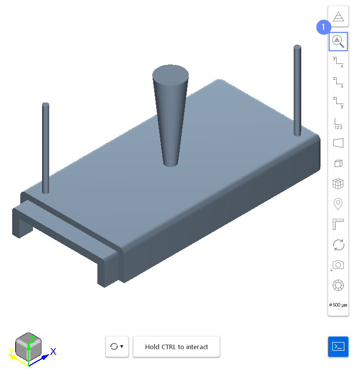
6. Geometry - Housing
After importing geometry, it will appear in the 3D view.
- Click Fit View to fit geometry in the view
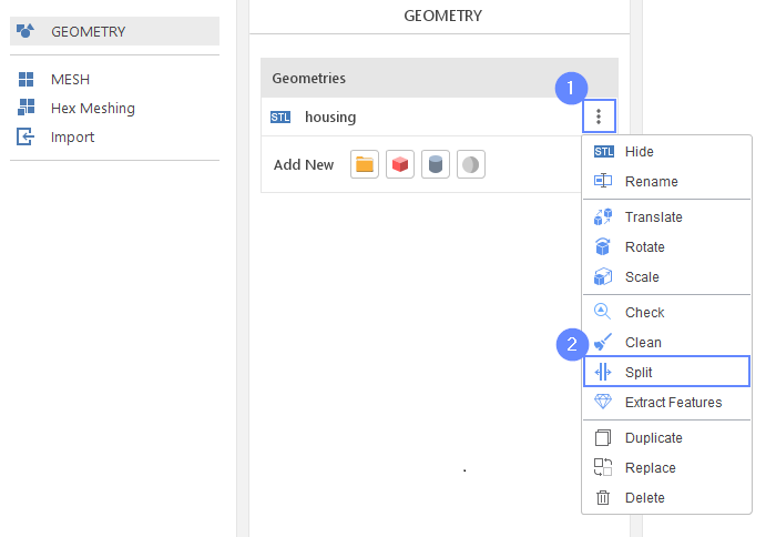
7. Split Geometry - Housing (I)
The imported geometry is made up of a single surface. We need to split it into separate faces for further processing.
- Expand the Options list
- Select Split
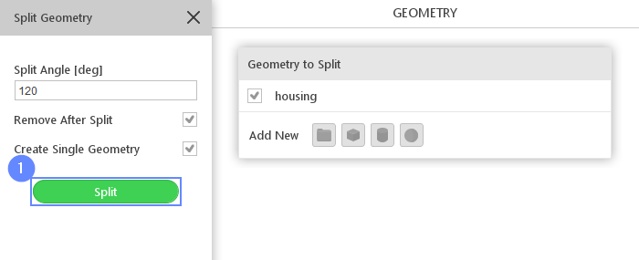
8. Split Geometry - Housing (II)
- Click Split
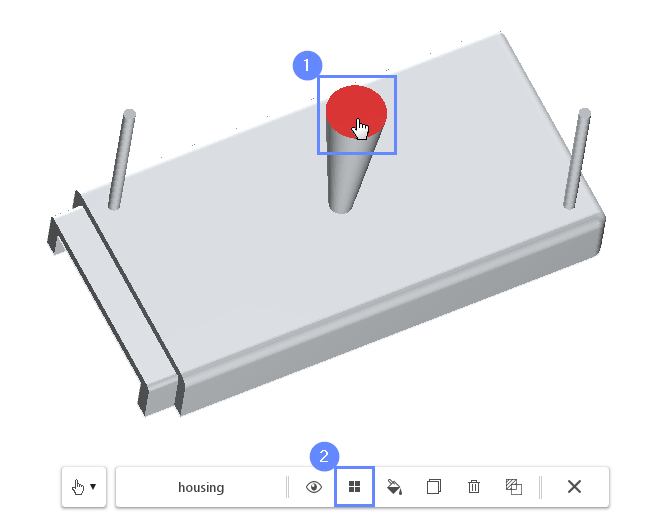
9. Create Face Groups (I)
We will add 3 face groups to the original geometry. SimFlow treats each face group as a mesh boundary. By using face groups, we can create separate boundaries for inlet and outlets.
- Select the inlet face by holding CTRL button and clicking on the geometry face
- Press Create face group from selection button
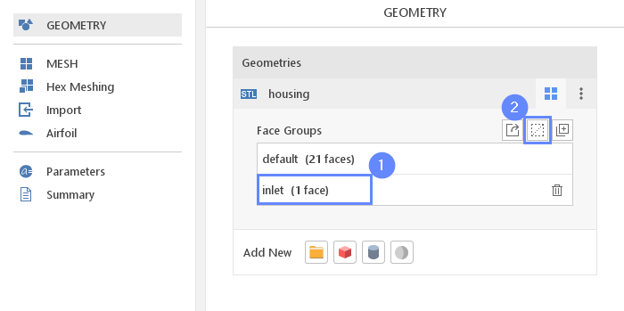
10. Create Face Groups (II)
New component should be appeared on the Face Groups list.
- Change face group name from group_1 to inlet
(double click to edit name and press Enter to confirm) - To uncheck the selected face from graphics click on Clear Selection or press the Esc key
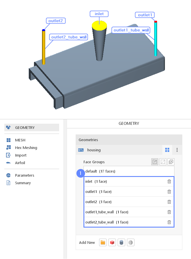
11. Create Face Groups (III)
Repeat this operation for the outlets. Additionally, we need to add outlet tube walls as separate groups to set the mesh refinement for these regions. Each group should contain a single face.
- Create and rename new groups as follows:
outlet1
outlet2
outlet1_tube_wall
outlet2_tube_wall
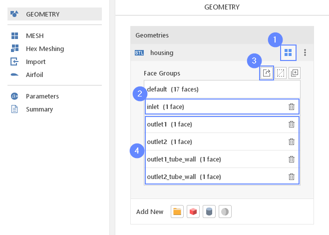
12. Create Face Groups (IV)
In order to be able to set different settings per each face, we will convert the single geometry into multiple geometry objects.
- Select Geometry Faces
- Click on the inlet group
- Click on Extract group
- Repeat this operation for the rest of created face groups
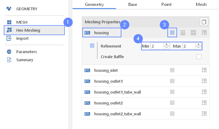
13. Meshing Parameters - Housing
Before we start meshing we will specify geometry options used during the meshing. We will also increase the refinement level for better accuracy.
- Go to Hex Meshing panel
- Select the housing component
- Enable Mesh Geometry
- Set Refinement to Min 2 Max 2
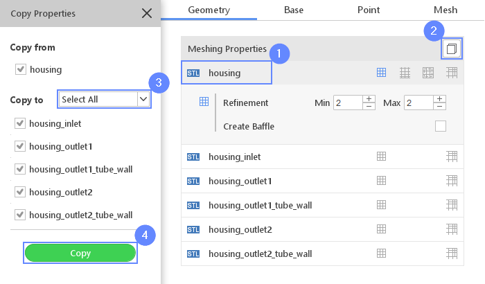
14. Copy Meshing Parameters
We will use the copy option to apply common settings.
- Select housing
- Click on Copy Meshing Properties
- Select all remaining faces as a target
- Click on Copy
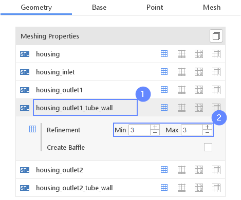
15. Meshing Parameters - Housing Outlet 1 Tube Wall
For outlet tubes, we will increase copied refinement levels.
- Select the housing_outlet1_tube_wall
- Increase the Refinement to Min 3 Max 3
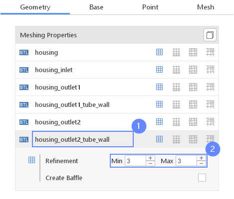
16. Meshing Parameters - Housing Outlet 2 Tube Wall
- Select the housing_outlet2_tube_wall
- Increase the Refinement to Min 3 Max 3
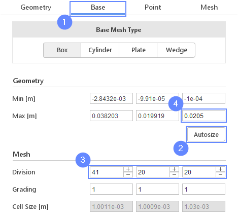
17. Base Mesh - Domain
Under the Base tab we will define the background mesh for the housing.
- Go to Base tab
- Click on Autosize
- Set the division of the base mesh
Division412020 - Change Max [m] Z to 0.0205
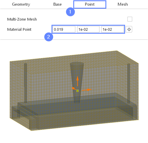
18. Material Point
Material Point tells the meshing algorithm on which side of the geometry the mesh is to be retained. Since we are considering flow inside the housing we need to place the material point inside the geometry.
- Go to Point tab
- Specify location inside housing geometry
Material Point0.0191e-021e-02
You can specify the point location from the 3D view. Hold the CTRL key and drag the arrows to the destination.
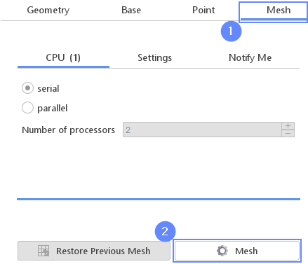
19. Start Meshing
- Switch to Mesh tab
- Start the meshing process with Mesh button
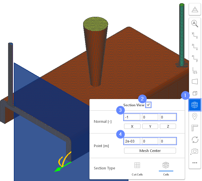
20. Check Mesh - Section View (I)
After the meshing process is finished the mesh should appear in the graphics window. In order to check the quality of the mesh, we view the element’s shape using section view.
- Select Section View from panel
- Check the Section View
- Set the normal vector to the section plane
Normal \({\sf [-]}\)-100 - Set the point to set the location of section plane
Point \({\sf [m]}\)2e-0300
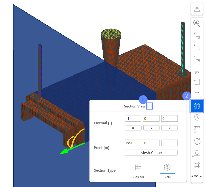
21. Check Mesh - Section View (II)
After the mesh check, we will turn off the section view to return to the full model view.
- Uncheck the Section View
- Click Section View options or press ESC key to close panel
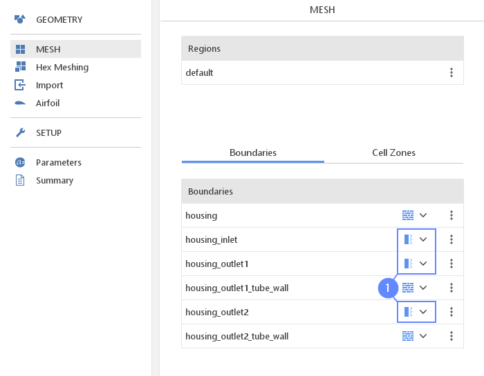
22. Mesh - Boundaries
To be able to assign inlet and outlet boundary conditions we have to adjust the boundary types.
- Set the boundary type to Patch for inlet and outlets boundaries
inlet Patch
outlet1 Patch
outlet2 Patch
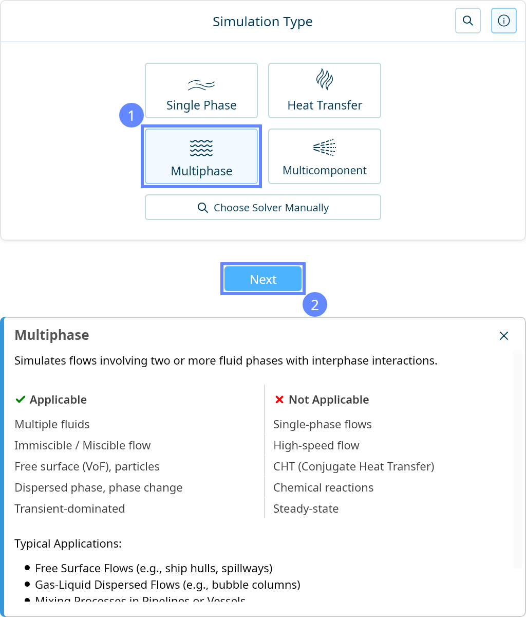
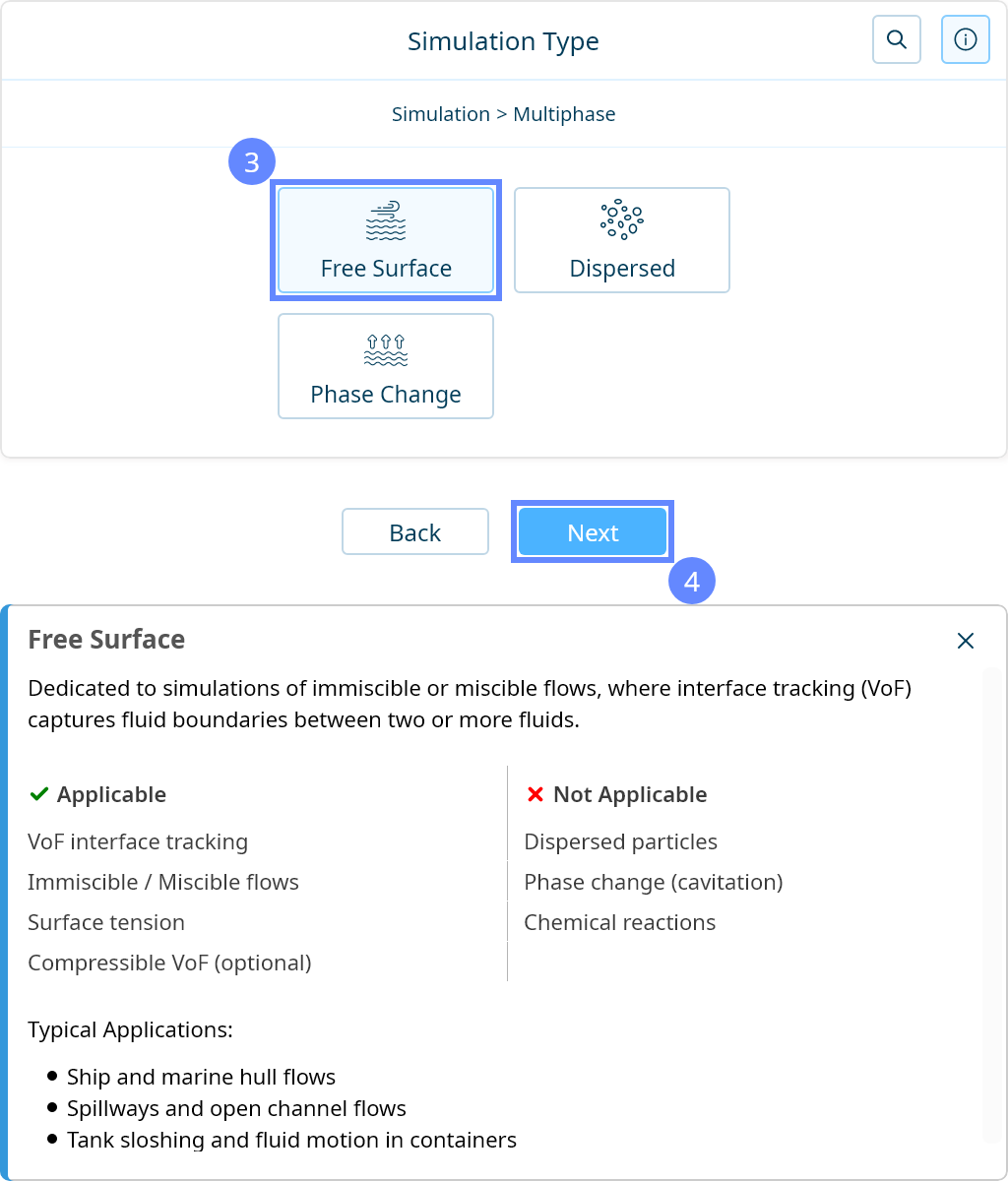
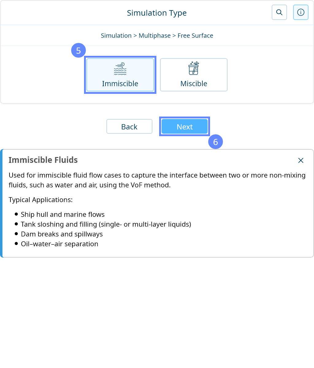
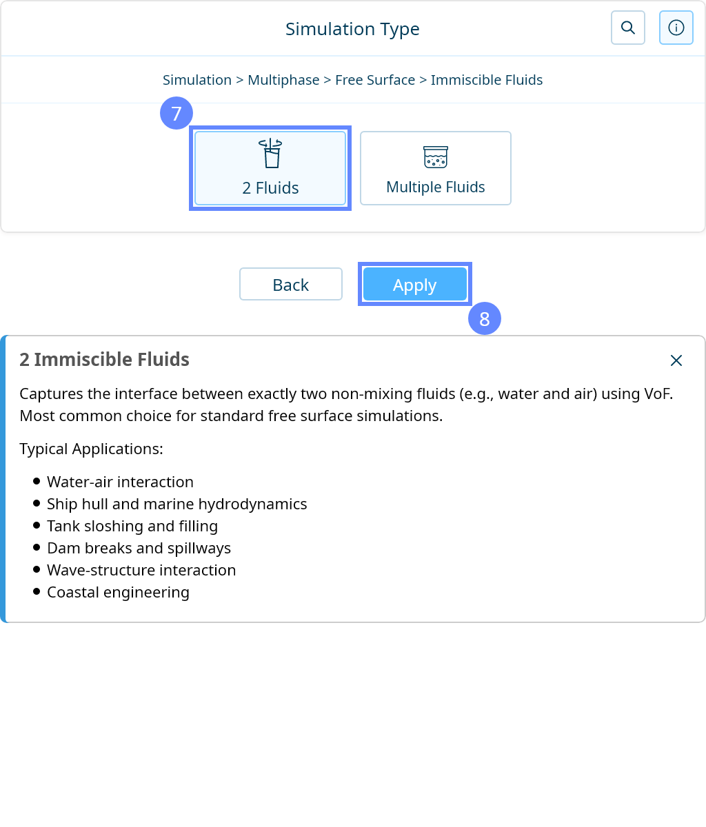
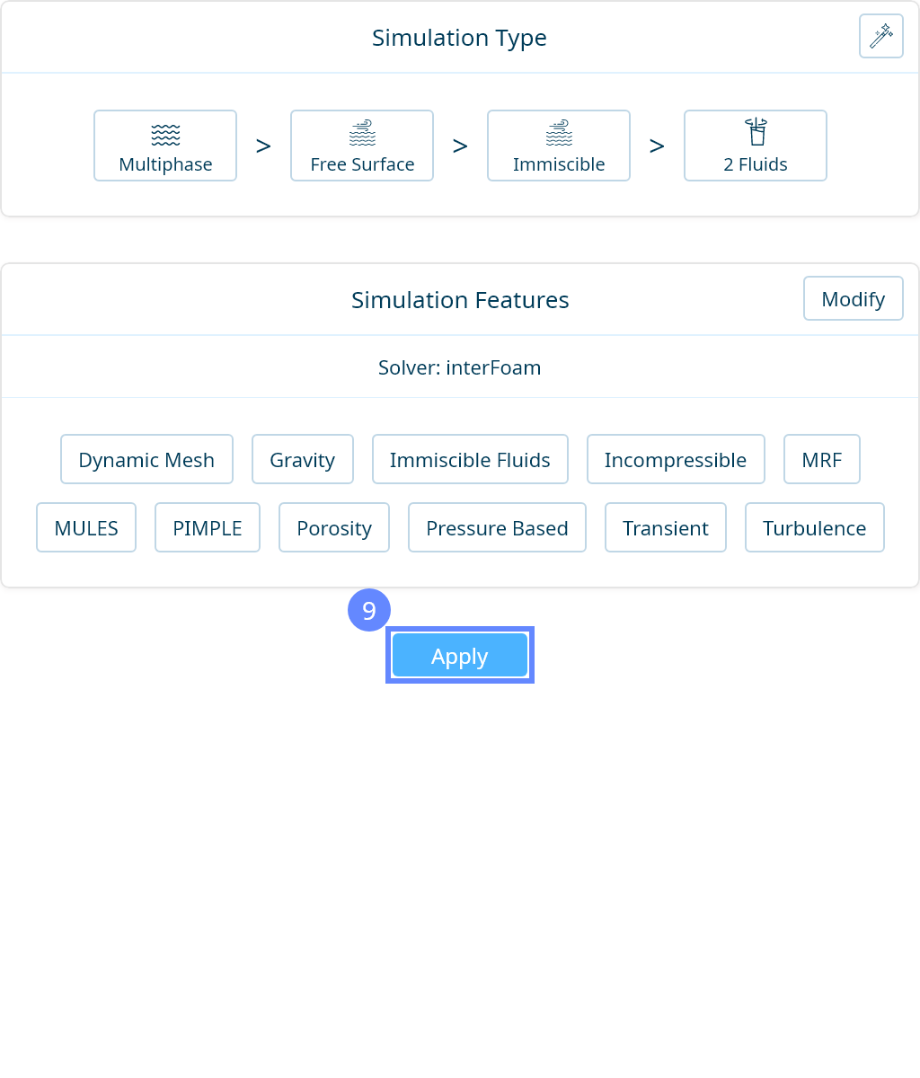
23. Simulation Type
We want to analyze the filling process in injection molding. For this purpose, we will use a transient simulation of two immiscible fluids (filament and air) using the free-surface method.

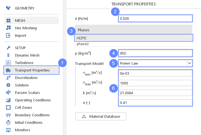
24. Transport Properties - HDPE
In the transport properties panel, we will define fluid parameters. Firstly, we will define High-Density Polyethylene (HDPE) phase using Power Low transport model.
- Go to Transport Properties panel
- Set the surface tension between fluids
\(\sigma\) \({\sf [N/m]}\)0.026 - Change phase name from phase1 to HDPE
- Set the density
\(\rho\) \({\sf [kg/m^3]}\)952 - Extend the list for Transport Model and choose Power Law
- Set the parameters accordingly
\(\nu_{min}\) \({\sf [m^2/s]}\)6e-03
\(\nu_{max}\) \({\sf [m^2/s]}\)1000
\(k\) \({\sf [m^2/s]}\)21.0084
\(n\) \({\sf [-]}\)0.41
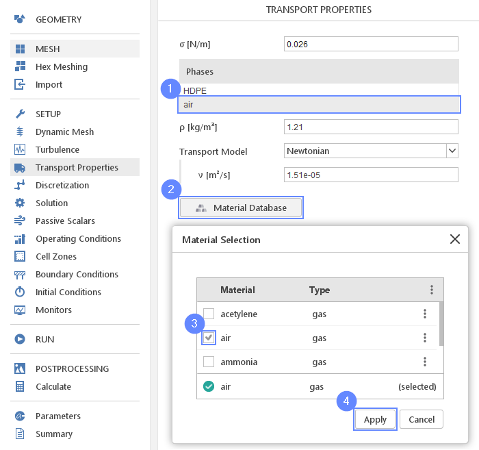
25. Transport Properties - Air
For the second phase, we will use predefined air properties from the material database.
- Change phase name from phase2 to air
- Click on Material Database
- Select the air
- Click Apply
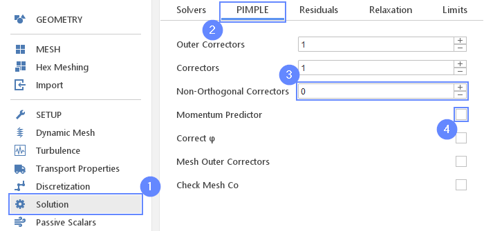
26. Solution - PIMPLE
For the purpose of the simulation, we will change the default PIMPLE algorithm parameters.
- Go to Solution panel
- Switch to the PIMPLE tab
- Set Non-Orthogonal Correctors to 0
- Uncheck Momentum Predictor for stability
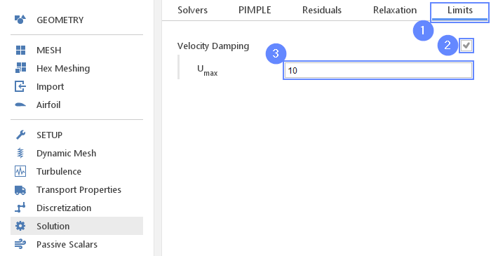
27. Solution - Limits
During computations sometimes velocity can spontaneously approach unphysical values due to numerical errors. In order to prevent computations from divergence, we can limit the velocity. As the result, we should get more stable computations.
- Switch to the Limits tab
- Check Velocity Damping
- Set the maximum velocity \(U_{max}\) to 10
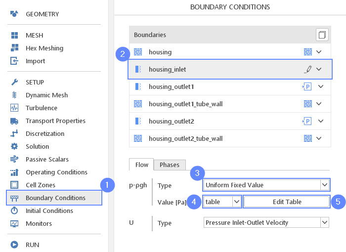
28. Boundary Conditions - Inlet (Flow I)
In order to define injection, we will use pressure inlet boundary. We will define the pressure by time history table.
- Go to Boundary Conditions panel
- Select housing_inlet
- Change the pressure type to Uniform Fixed Value
- Set the Value [Pa] as table
- Press Edit Table
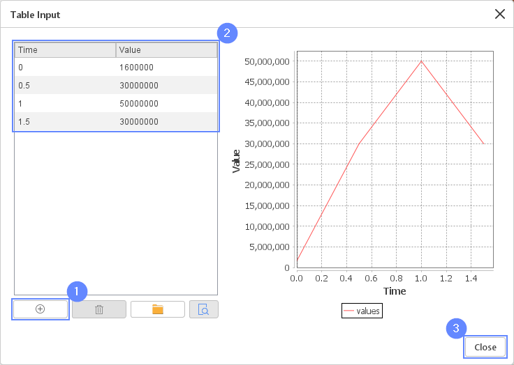
29. Boundary Conditions - Inlet (Flow II)
Fill in inlet pressure values history.
- Press Add Row two times
- Fill the table by values
01600000
0.530000000
150000000
1.530000000 - Close the window
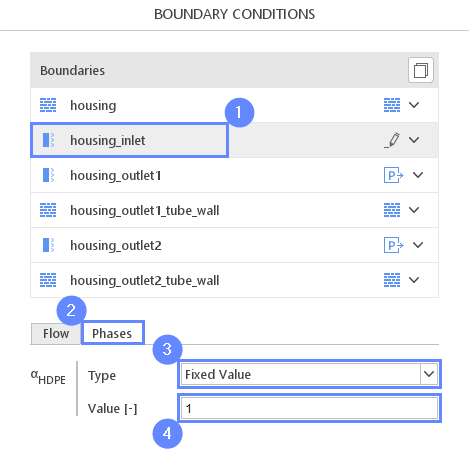
30. Boundary Conditions - Inlet (Phases)
To assign injected material, the phase fraction parameter \(\alpha_{phase}\) is used. \(\alpha_{HDPE}\) equal 1 will stand for HDPE phase.
- Select housing_inlet
- Switch to the Phases tab
- Set the Type to Fixed Value
- Set the Value [-] to 1
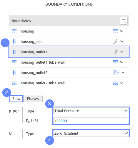
31. Boundary Conditions - Outlet (Flow I)
Outlets' boundary conditions simulate outflow to the atmosphere. The default phase setup allows both fluids to exit freely while in case of backflow only air can be sucked into the housing.
- Select housing_outlet1
- Switch the tab to Flow
- Set the pressure type and its value accordingly
\(p{-}\rho gh\)TypeTotal Pressure
\(p{-}\rho gh\)\(p_0\) \({\sf [Pa]}\)100000 - Change the velocity Type to Zero Gradient
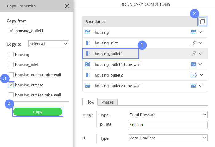
32. Boundary Conditions - Outlet (Flow II)
We will copy the boundary condition settings to the second outlet.
- Select housing_outlet1
- Press Copy Boundary Conditions
- Check the housing_outlet2
- Press Copy
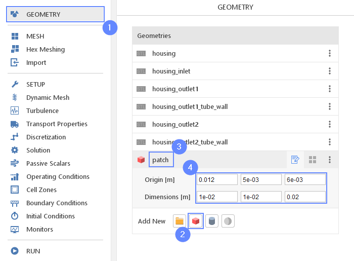
33. Create Geometry - Patch
Before we will set the initial condition we need to define the region representing the initial location of HDPE. For this purpose, we will create a box.
- Go to GEOMETRY panel
- Select Create Box
- Change geometry name from box_1 to patch
- Set the origin and box dimensions
Origin \({\sf [m]}\)0.0125e-036e-03
Dimensions \({\sf [m]}\)1e-021e-020.02
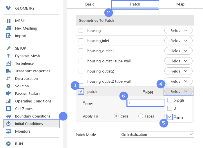
34. Initial Conditions - Patch
By using the previously created geometry we will tell the solver where should be localized HDPE at the initial state.
- Go to Initial Conditions panel
- Switch to Patch tab
- Check the patch geometry
- Expand the Fields
- Check \(\alpha_{HDPE}\)
- Override \(\alpha_{HDPE}\) with the value of 1
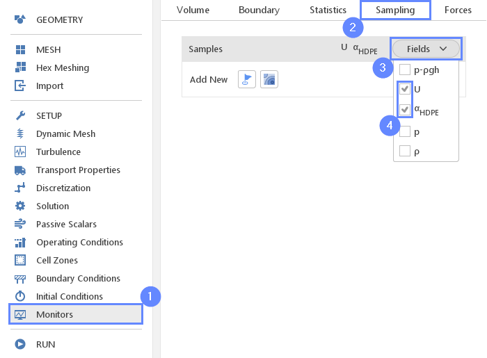
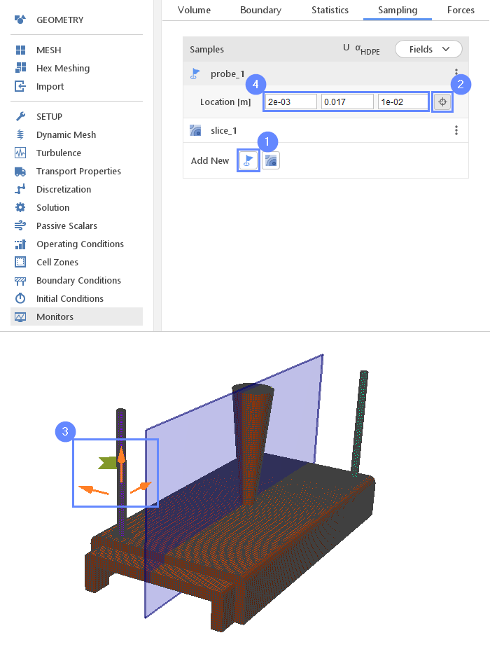
35. Monitors - Sampling
During calculation, we can observe intermediate results on a section plane or probe plots. Note that runtime post-processing can only be defined before starting calculations and can not be changed later on. Firstly, we need to specify variables that will be sampled. After that, we will define the section plane and probes.
- Go to Monitors panel
- Switch to Sampling tab
- Expand Fields list
- Select the velocity U and the HDPE phase \(\alpha_{HDPE}\)
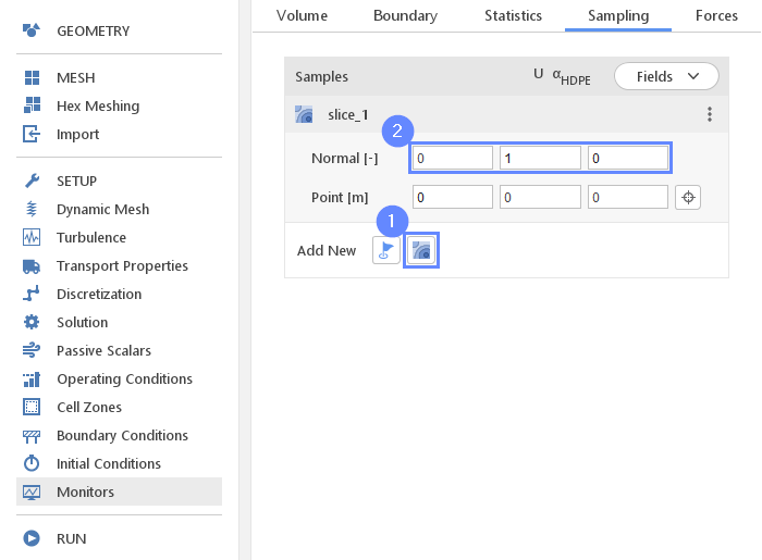
36. Monitors - Create Slice (I)
To add sampling data on a plane we need to create a slice. To define a plane we need to set the normal vector and then select the point. In the current step, we will choose the normal vector and in the next step, we will choose a point that belongs to the plane.
- Select Create Slice
- Set the normal along Y axis
Normal \({\sf [-]}\)010
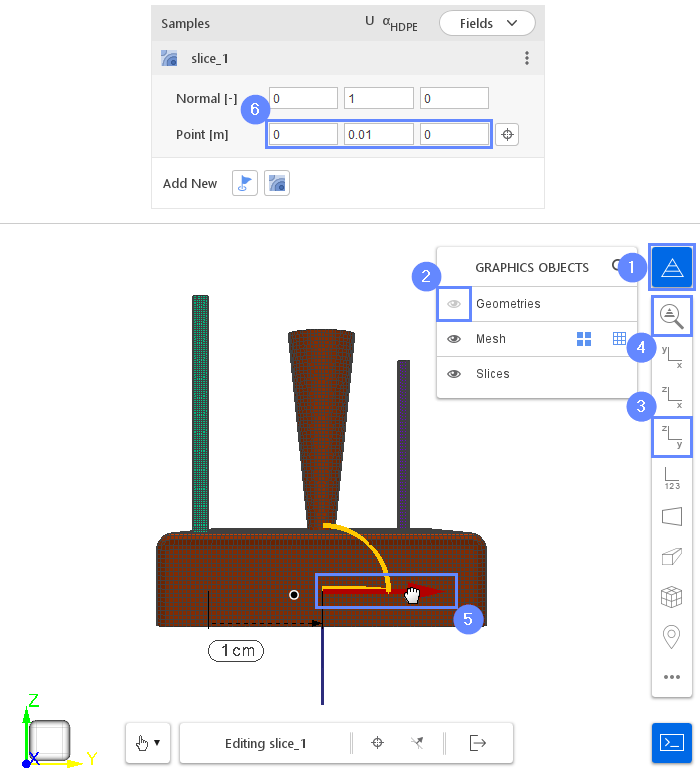
37. Monitors - Create Slice (II)
Now we will place the slice to the destination by setting the point coordinates. To achieve this we will use arrows in the graphic window. Before that, we will hide unnecessary geometries.
- Extend Graphic Objecyt List
- Uncheck Geometries
- Set YZ View orientation
- Click Fit View
- Holding CTRL button, click on the red arrow and drag it to the middle of the model
- The slice point coordinates should be like this
Point00.010
38. Monitors - Create Probe
To track sampled parameters in a specific point in space, we can add the probe location monitor.
- Add New Probe
- Press the viewfinder icon next to Location [m] coordinates
- Set the probe location on the 3D view. Holding CTRL button, move the probe to the specific location
- The probe point location should be like this
Location \({\sf [m]}\)2e-030.0171e-02
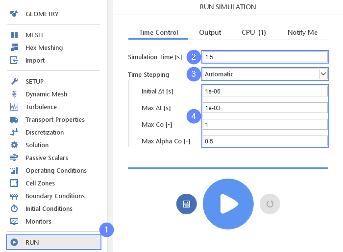
39. Run - Time Control
For any simulation, it is very convenient to let the solver automatically determine the proper time step value. To use this option we need to define time step constraints by providing the initial time step (adjusted by the solver during computations), maximal time step value and Courant number.
- Go to RUN panel
- Set the Simulation Time [s] to 1.5
- Change Time Stepping to Automatic
- Set the parameters:
Initial \(\Delta t\) \({\sf [s]}\)1e-06
(solver will start computation with this value and adjust it in the next iterations)
Max \(\Delta t\) \({\sf [s]}\)1e-03
Max Co \({\sf [-]}\)1
Max Alpha Co \({\sf [-]}\)0.5
This calculation will require high CPU usage and might take several hours to finish the calculation depending on the machine used. If you want to shorten the computation time, you can decrease the Simulation Time to 0.4s - this is enough for purpose of further postprocessing.
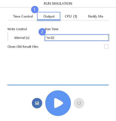
40. Run - Output
We can control how often results should be saved on the hard drive. Only this data will be available for postprocessing.
- Switch to Output tab
- Set the Interval [s] to 1e-02
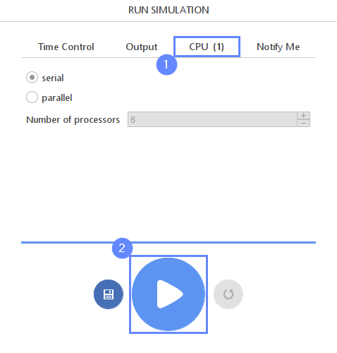
41. Run - CPU
To speed up the calculation process, take advantage of parallel computing and increase the number of CPUs based on your PC’s capability. The free version allows you to use only one processor (serial mode). To get the full version, you can use the contact form to Request 30-day Trial
Estimated computation time for serial mode: over 5 hours
- Switch to CPU tab
- Click Run Simulation button
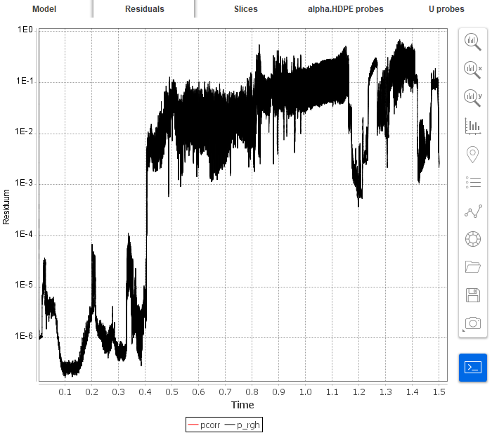
42. Monitor Solution - Residuals
When the calculation is finished we should see a similar residual plot.
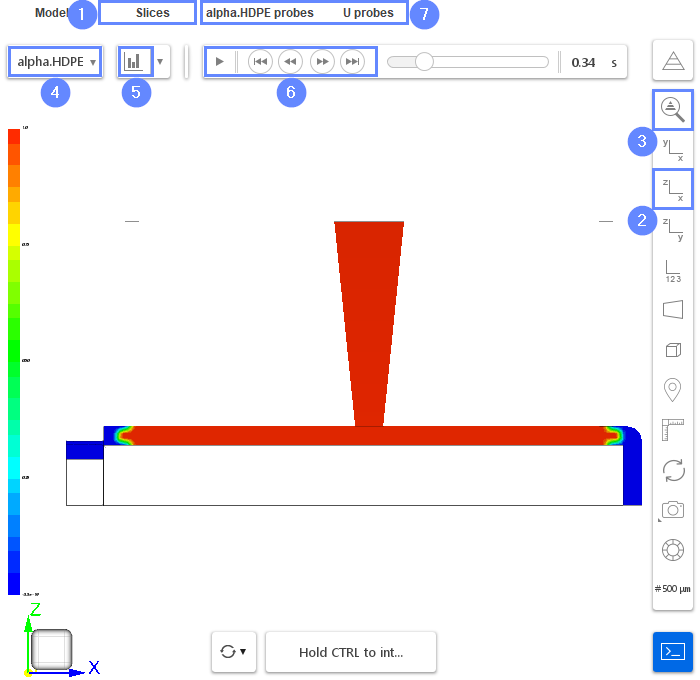
43. Results - Slice
Slices tab appears next to Residuals. Under this tab, we can preview results on the defined slice planes. The results preview is available during the calculation and we can track it on a regular basis. The newly calculated time step will be actualized automatically as long as the time selector points to the latest time step.
- Switch to Slices tab
- Click ViewXY
- Click Fit View to zoom the geometry
- Choose alpha.HDPE field
- Click Adjust range to data
- Play with an animation buttons to track the results of analysis
- Probes outputs are available to preview on the sheets next to Slice
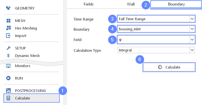
44. Calculate - Mass Flow
After computations are finished, we will investigate the mass flow rate during the injection. We will compute it by using already existing data (this feature is not available as a monitor).
- Go to Calculate panel
- Switch to Boundary tab
- Select Full Time Range
- Select the boundary as housing_inlet
- Select mass \(\varphi\)
- Click on Calculate
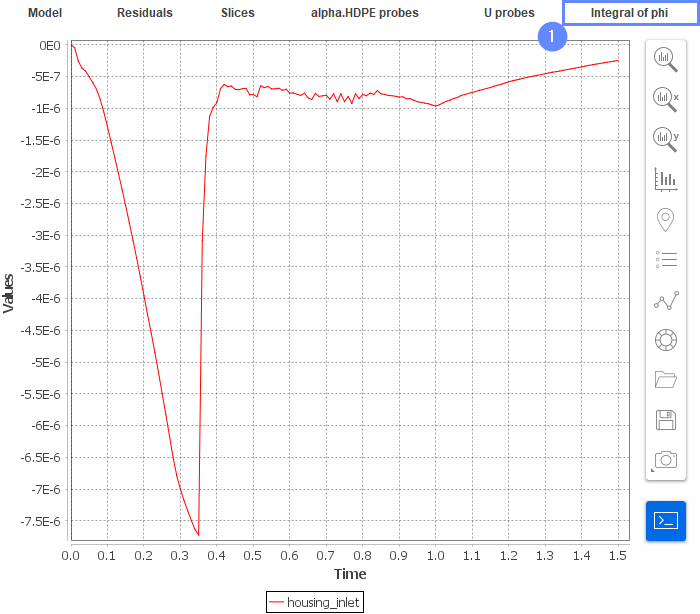
45. Results - Mass Flow
- Computed variables are displayed on the chart in the tab Integral of phi
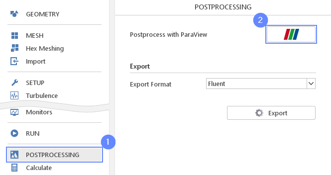
46. Postprocessing - ParaView
We can do the complex visualization of our results with ParaView.
- Go to POSTPROCESSING panel
- Click on Run ParaView
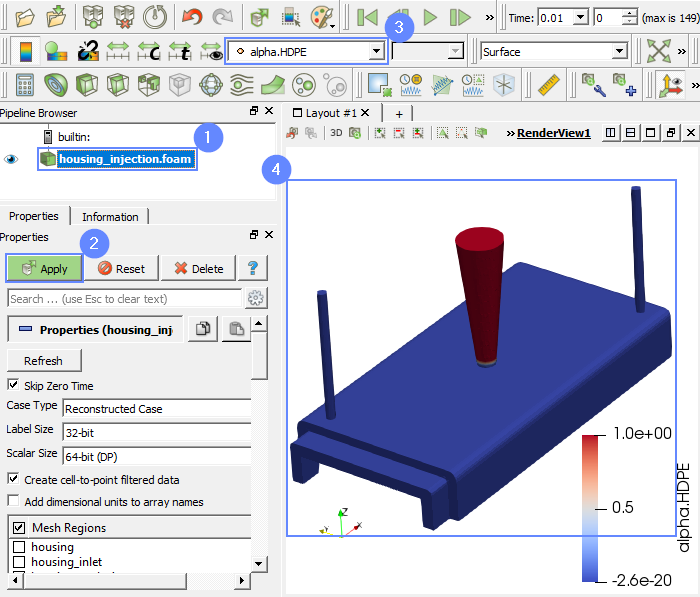
47. ParaView - Load the results
Load the results into the program.
- Mark housing_injection.foam
- Click Apply to load results into ParaView
- Select the phase alpha.HDPE from the list
- After loading results they will be shown in the 3D graphic window
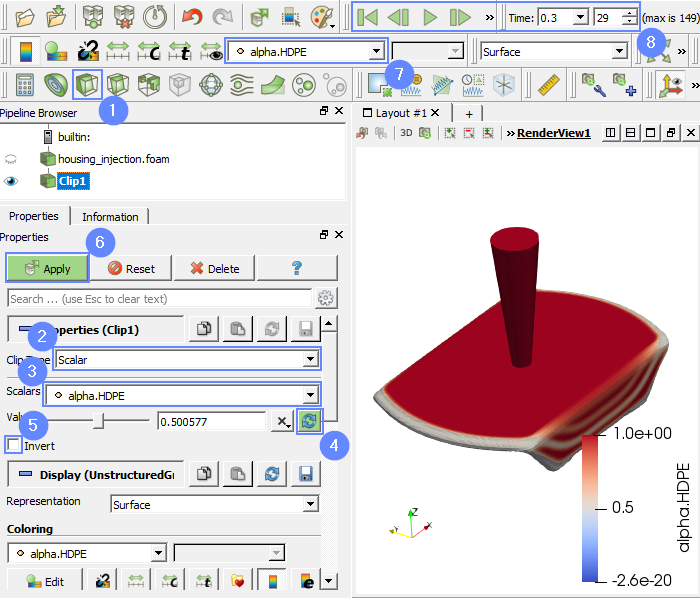
48. ParaView - Results (I)
We will focus on the HPDE phase behavior and observe form filling during the injection.
- Select Clip from top menu
- Change the clip type to Scalar
- Select alpha.HDPE from the scalar list
- Click Refresh
- Uncheck Invert option
- Click Apply
- Select the phase alpha.HDPE to preview
- Play with the animation buttons to track the HDPE phase movement
49. ParaView - Results (II)
To show the housing together with the fluids we will follow these steps
- Unhide housing_injection.foam
- Set the coloring by the Solid Color
- Set the opacity to 0.3
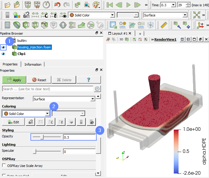
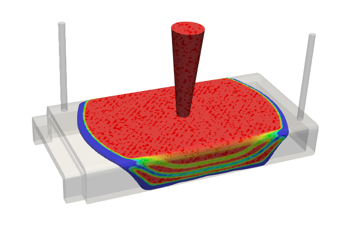
50. Final Results
Now we can see the final results with the original geometry.