3. Create Case
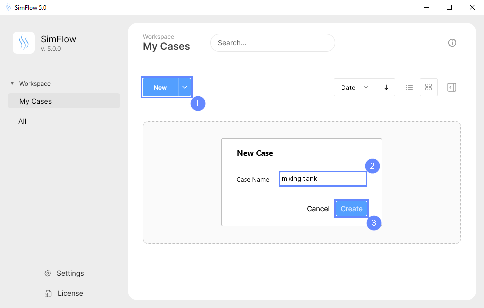
Open SimFlow and create a new case named mixing tank
- Click New
- Provide name mixing tank
- Click Create to open a new case
4. Import Geometry
After creating case Download GeometryImpeller
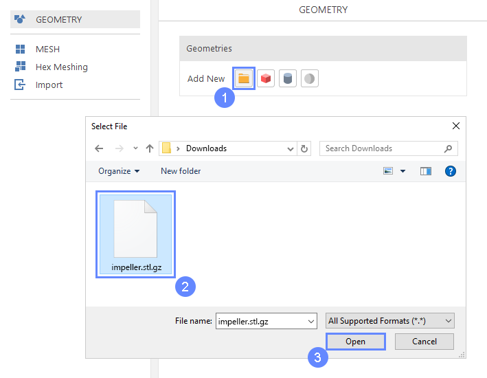
- Click Import Geometry
- Select geometry file impeller.stl.gz
- Click Open
5. Imported Geometry Units
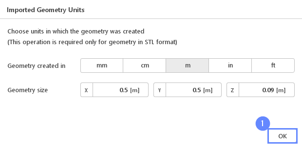
In a next step we need to select the unit in which the model was exported. The STL format does not contain the unit information which are defined during the geometry export. The Geometry size displays the overall size of the model what allows to select the suitable unit. In this case, the default unit meter is correct.
- To confirm default unit meter, press OK
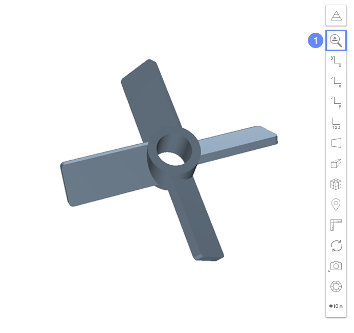
6. Geometry - Impeller
After importing geometry, it will appear in the 3D window.
- Click Fit View to zoom the geometry
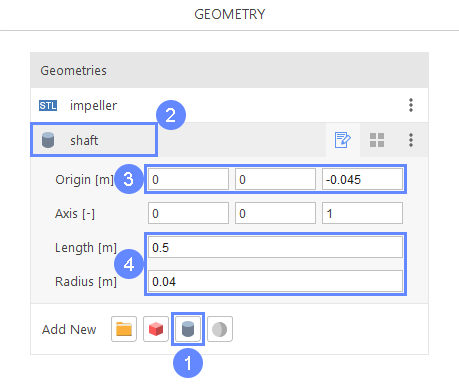
7. Create Geometry - Shaft
The original impeller geometry consists of only blades. To make the impeller complete we will add a shaft using a primitive geometry.
- Click Create Cylinder
- Rename cylinder_1 to shaft
(double click on the geometry name to start rename) - 4 Define cylinder origin, length, and radius
Origin \({\sf [m]}\)00-0.045
Length \({\sf [m]}\)0.5
Radius \({\sf [m]}\)0.04
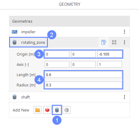
8. Create Geometry - Rotating Zone
We want our impeller to be rotating. We will create a cylindrical zone that will be used to divide the mesh into rotating and stationary part.
- Click Create Cylinder
- Rename cylinder_1 to rotating_zone
- 4 Define cylinder origin, length, and radius
Origin \({\sf [m]}\)00-0.105
Length \({\sf [m]}\)0.6
Radius \({\sf [m]}\)0.3
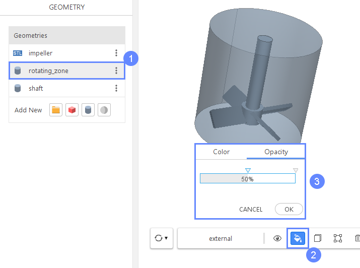
9. Show Impeller
All parts of the geometry are displayed in the graphics window now. Note that rotating_zone encloses the impeller and shaft. In order to see all geometries, we will decrease the opacity of the rotating_zone.
- Press Esc to exit edit mode then select rotating_zone if it is not selected
- Click Display Properties
- Adjust Opacity to 50%
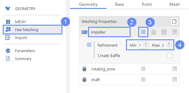
10. Meshing Properties - Impeller
We will enable meshing for impeller geometry.
- Go to Hex Meshing panel
- Select impeller
- Check Mesh Geometry
- Set Refinement to Min 1 Max 2
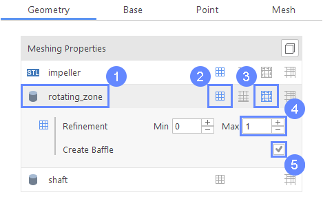
11. Meshing Properties - Rotating Zone
Since our domain will consist of a stationary and a rotating part we need to create a mesh interface between the parts. To do this we will create a baffle using the rotating_zone geometry.
- Select rotating_zone
- Check Mesh Geometry
- Check Create Cell Zone
- Change Refinement Max level to 1
- Check Create Baffle
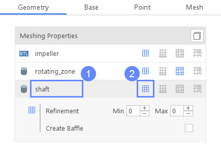
12. Meshing Properties - Shaft
We need to also mesh the shaft geometry.
- Select shaft
- Check Mesh Geometry
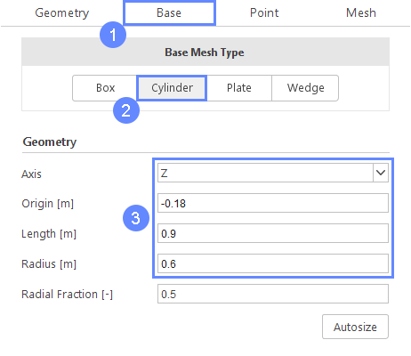
13. Base Mesh - Geometry
Now we will define the outer bounds of the computational domain.
- Go to Base tab
- Select Cylinder as the base mesh type
- Define cylinder axis, origin, length, and radius
AxisZ
Origin \({\sf [m]}\)-0.18
Length \({\sf [m]}\)0.9
Radius \({\sf [m]}\)0.6
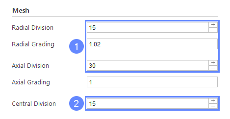
14. Base Mesh - Mesh
To have an appropriate mesh density we will use the following divisions and grading of the base mesh.
- 2 Define radial division, radial grading, axial division, and central division
Radial Division15
Radial Grading1.02
Axial Division30
Central Division15
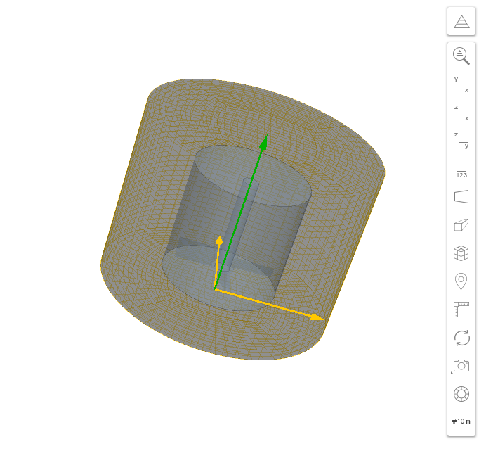
15. Base Mesh - View
We can preview the Base Mesh in the graphics window.
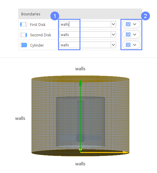
16. Base Mesh - Boundaries
Now we need to assign individual names to each side of the base mesh. Since we are modeling a closed tank all our boundaries will be defined as walls.
- Type boundary names accordingly
First Disk walls
Second Disk walls
Cylinder walls - Change type of all boundaries to wall
First Disk wall
Second Disk wall
Cylinder wall
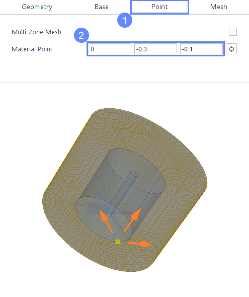
17. Material Point
Material Point tells the meshing algorithm on which side of the geometry the mesh is to be retained. Since we are modelling flow inside the tank we need to place the material point between the tank walls and the propeller.
- Go to Point tab
- Specify location inside the mesh
Material Point0-0.3-0.1
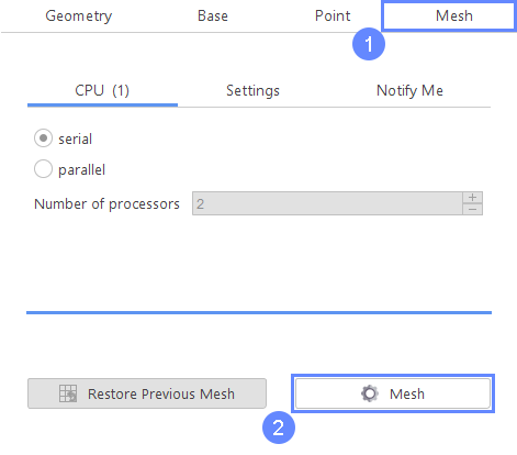
18. Meshing
Everything is now set up for meshing.
- Go to Mesh tab
- Click Mesh button to start meshing process
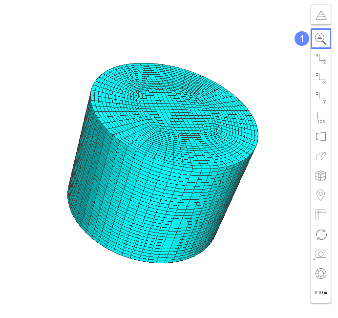
19. Mesh
After the meshing process is finished the mesh will appear in the 3D graphics window. The mesh used in this tutorial is created for demonstration purposes only, and its resolution should be considerably finer in real case scenario.
- Click Fit View to zoom the geometry
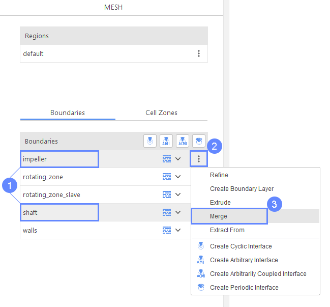
20. Merge Boundaries - Impeller and Shaft (I)
In order to simplify the definition of boundary conditions, we will merge the shaft and propeller boundaries into a single boundary.
- Hold CTRL key and select impeller and shaft boundaries
- On the impeller boundary select Options
- Choose Merge operation from the dropdown menu
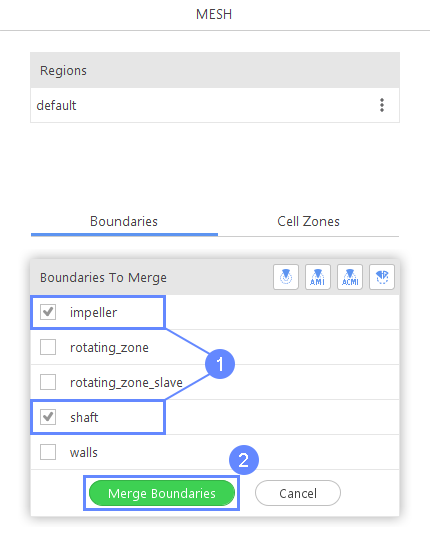
21. Merge Boundaries - Impeller and Shaft (II)
- Make sure you have selected impeller and shaft boundaries
- Click Merge Boundaries to confirm the operation
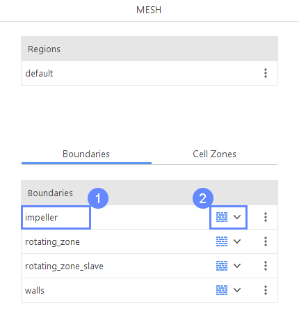
22. Merge Boundaries - Impeller and Shaft (III)
- Rename newly created boundary from impeller_merged to impeller
- Change impeller’s boundary type to wall
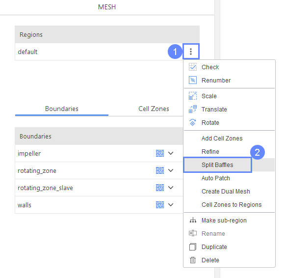
23. Split Baffles
Even though we requested the creation of baffles for the rotating_zone, two sides of the baffle can still share some common nodes. In order to make sure that each side has its own nodes, we need to perform the Split Baffles operation on the mesh. This is a very important step when using dynamic mesh model.
- Expand Options of the default region
- Select Split Baffles from the drop-down list
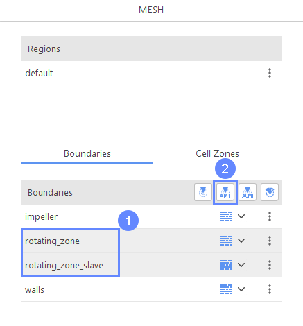
24. Create Mesh Interface
In the mesh setup, we requested creating baffles for rotating_zone, so that it can be a slip surface for the dynamic mesh. Now we will create the interface between the baffles.
- Hold CTRL key and select rotating_zone and rotating_zone_slave
- Click Create Arbitrary Interface
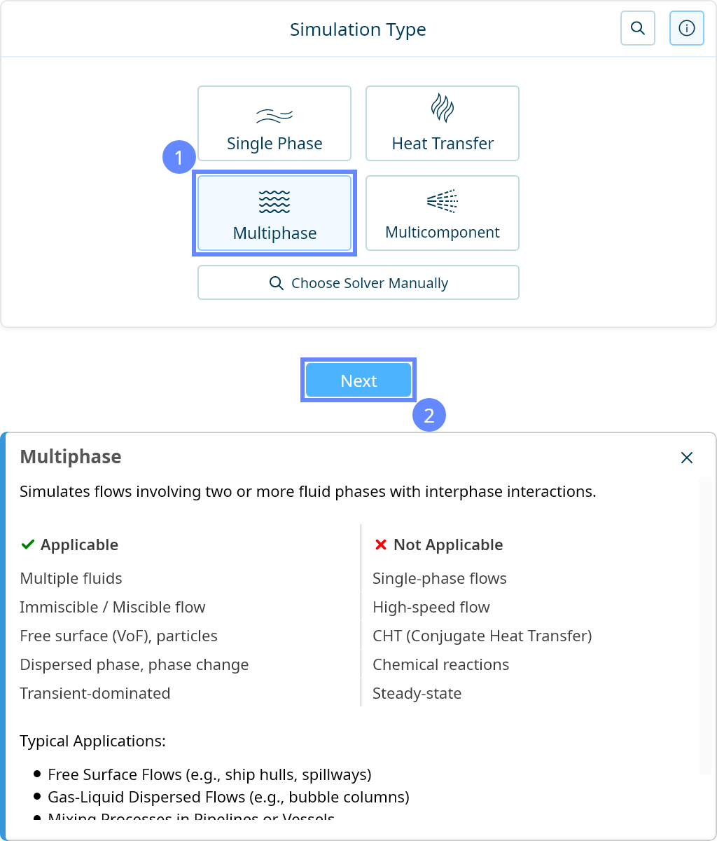
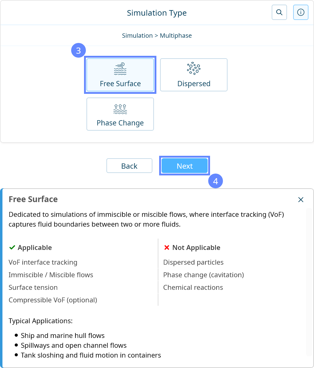
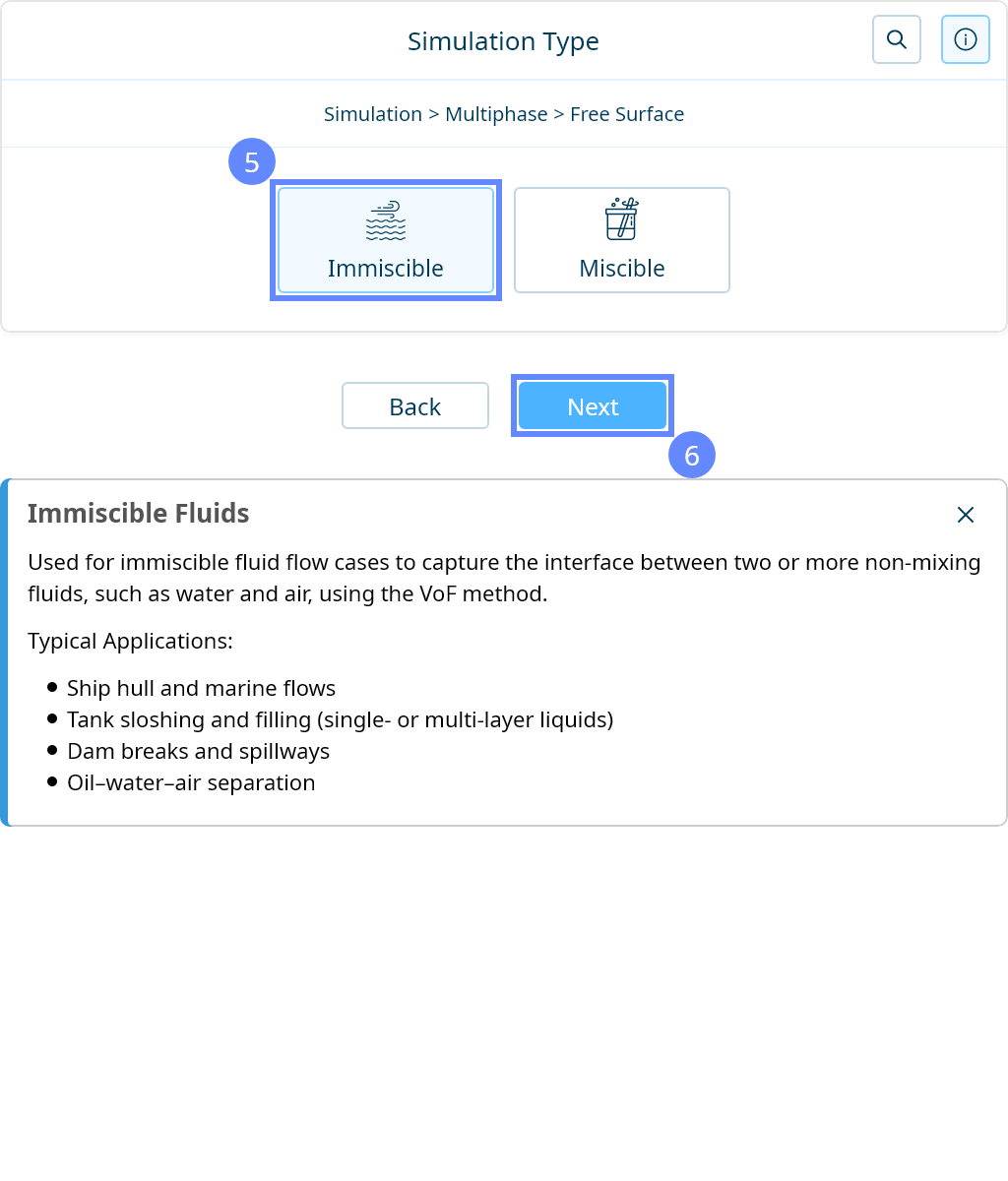
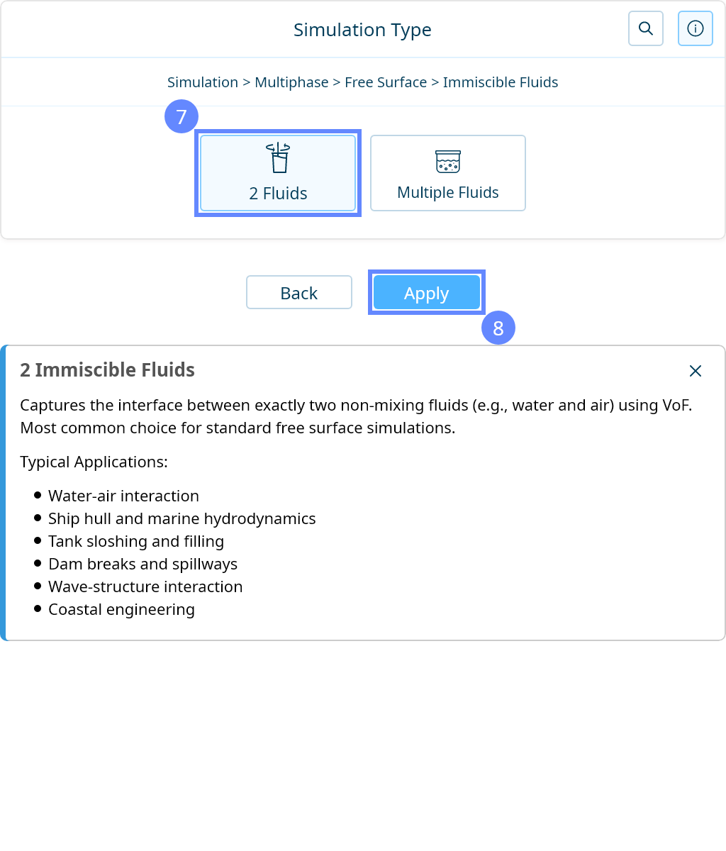
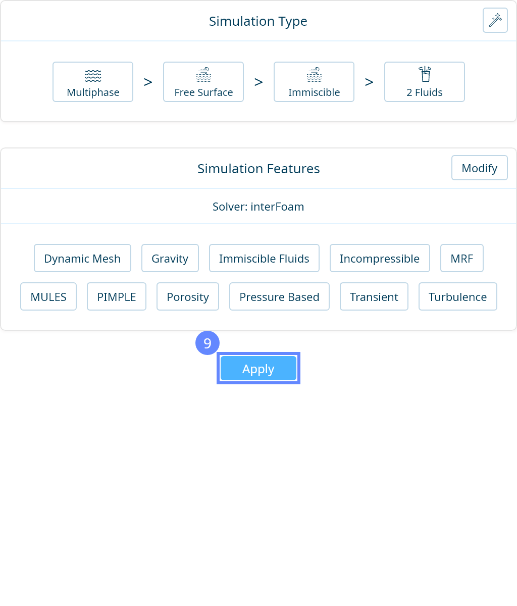
25. Simulation Type
We want to analyze the flow in a mixing tank with a rotating impeller. For this purpose, we will use a transient simulation of two immiscible fluids (water and air) using the free-surface method with dynamic mesh handling.

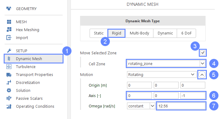
26. Dynamic Mesh
We will apply a rotational speed of 2 revolutions per second to the zone with the impeller. Due to the orientation of our geometry, our rotation axis will be the -Z-axis of the global coordinate system.
- Go to Dynamic mesh panel
- Select Rigid type
- Check Move selected zone
- Make sure rotating_zone is selected as Cell Zone
- Expand Motion options
- Set Axis \({\sf [-]}\)00-1
- Set rotational speed Omega \({\sf [rad/s]}\)12.56
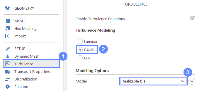
27. Turbulence
For turbulence modeling we will use \(Realizable \; k{-} \varepsilon\) model.
- Go to Turbulence panel
- Select RANS turbulence formulation
- Select \(Realizable \; k{-} \varepsilon\) model
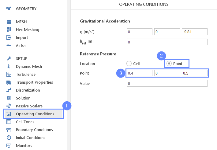
28. Operating Conditions
Incompressible solver like an Inter, operates on relative pressure (more here). In the incompressible Navier-Stokes equation, pressure is only related to the gradient and has no specific bounds. The pressure distribution can be determined by solving the N-S equation, but the exact value of pressure is irrelevant as long as the pressure difference between two points is the same.
To define precise value, it is necessary to define the pressure at a specific point. While the pressure at inlet or outlet boundaries is usually defined, if the domain is enclosed, a reference point must be established within the domain.
- Go to Operating Conditions panel
- Change the Location to Point
- Set Point0.400.5
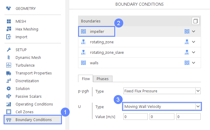
29. Boundary Conditions - Impeller (Flow)
We need to make sure that impeller velocity is taken from the properties of the rotating zone. For this purpose, we need to apply the Moving Wall Velocity boundary condition.
- Go to Boundary Conditions setup
- Select impeller boundary
- Change velocity type to Moving Wall Velocity
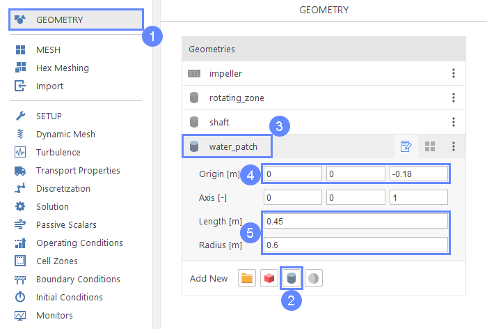
30. Geometry - Initial Conditions Patch
As an initial state, we want the mixing tank to be partly filled with water. For this purpose, we need to create geometry to indicate the initial water location.
- Go to Geometry panel
- Click Create Cylinder
- Rename cylinder_1 to water_patch
- 5 Define cylinder origin, length, and radius
Origin \({\sf [m]}\)00-0.18
Length \({\sf [m]}\)0.45
Radius \({\sf [m]}\)0.6
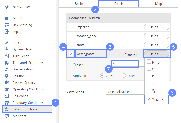
31. Initial Conditions - Patch
For initial conditions, we will leave all the default values, except inside the water patch, where the water phase fraction will be different.
- Go to Initial Conditions panel
- Switch to Patch tab
- Select water_patch geometry
- Enable initialization on water_patch
- Expand Fields list
- Select \(\alpha_{phase1}\) fraction for initialization
- Set \(\alpha_{phase1}\) to 1
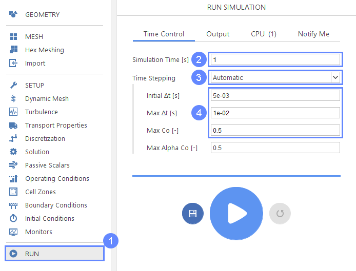
32. Run - Time Control
We will now adjust the time controls in order to capture the motion of the moving mesh in the output files. We will also enable automatic time step control for the simulation with reduced Courant number for better convergence.
- Go to Run panel
- Set Simulation Time [s] to 1
- Change Time Stepping to Automatic
- Set initial time step, time step limit and Courant number accordingly
Initial \(\Delta t\) \({\sf [s]}\)5e-03
Max \(\Delta t\) \({\sf [s]}\)1e-02
Max Co \({\sf [-]}\)0.5
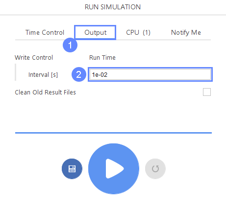
33. Run - Output
Now we just have to specify the frequency of writing results to the disk and start the simulation.
- Switch to Output panel
- Set Write Control Interval [s] to 1e-02
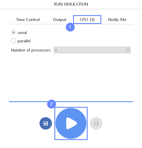
34. Run - CPU
To speed up the calculation process, take advantage of parallel computing and increase the number of CPUs based on your PC’s capability. The free version allows you to use only one processor (serial mode). To get the full version, you can use the contact form to Request 30-day Trial
Estimated computation time for serial mode: 50 minutes
- Switch to CPU tab
- Click Run Simulation button
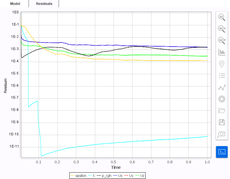
35. Residuals
When the simulation is finished we should see a similar residual plot.
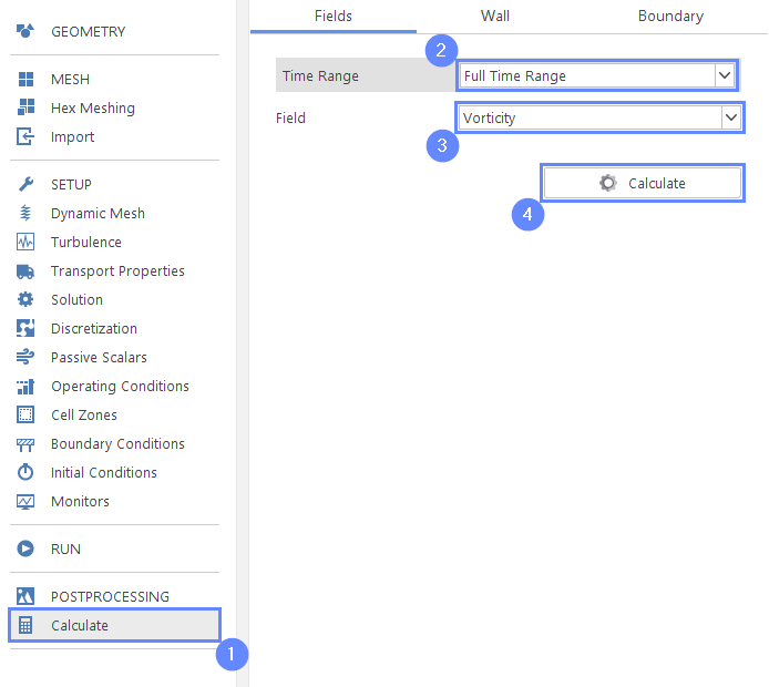
36. Calculate Additional Fields
When the simulation is finished we want to calculate additional flow variables to use later for postprocessing.
- Go to Calculate panel
- Select Full Time Range
- Select Vorticity field
- Click Calculate
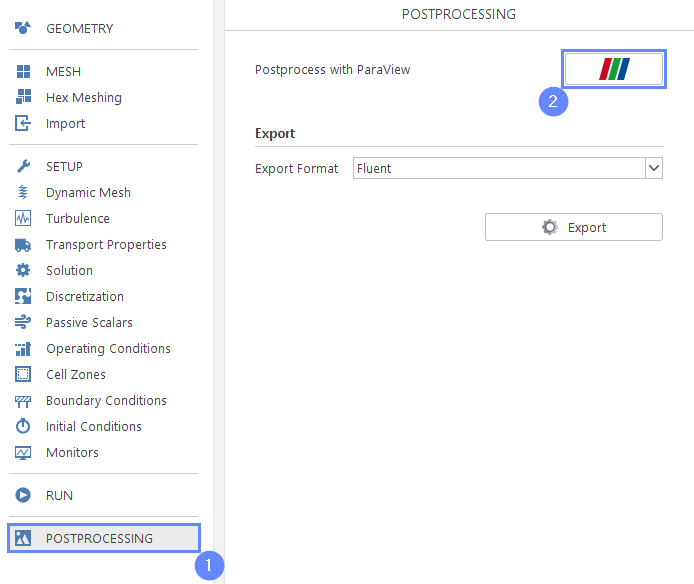
37. Start Postprocessing - ParaView
Start ParaView when the simulation is finished. Optionally you can start ParaView when the simulation is still in progress to observe the intermediate results.
- Go to Postprocessing panel
- Start ParaView
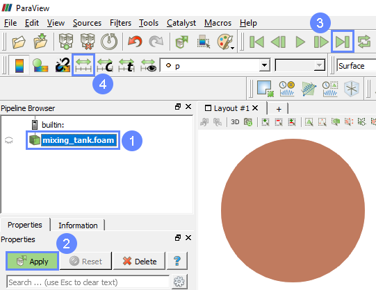
38. ParaView - Load Results
After opening ParaView, we have to load the results of the simulation.
- Select your case mixing_tank.foam
- Click Apply
- Click Last Frame
- Click Rescale to Data Range
- After rescale the contour will be shown in the 3D window.
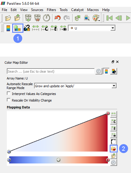
39. ParaView - Coloring (I)
We can change the coloring scheme in ParaView to have nicer colors.
- Click Edit Color Map from the menu placed on the left side, if the panel is not already shown.
- Select Choose Preset from the Color Map Editor placed by default on the right side of the ParaView
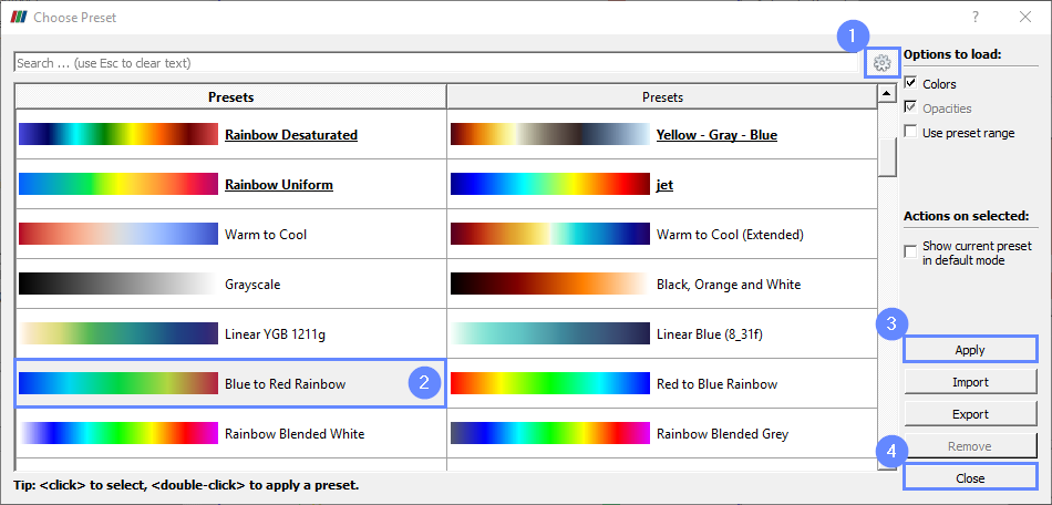
40. ParaView - Coloring (II)
We can now select a new Color Preset.
- Expand Advanced Options
- Choose Blue to Red Rainbow preset
- Apply changes
- Close Choose Preset window
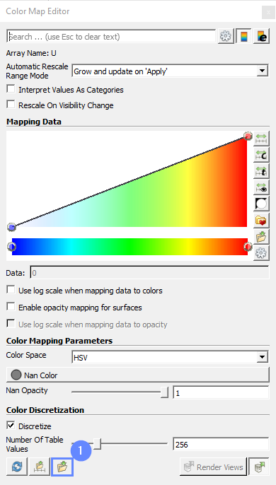
41. ParaView - Coloring (III)
To use the same color preset for all variables, we will save the current choice.
- Click Save current color map settings values as default for all arrays
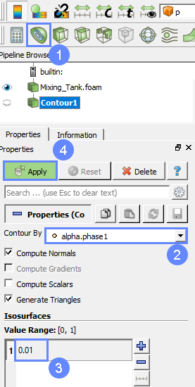
42. ParaView - Display Water Surface (I)
We will now plot the water surface colored by the water height.
- Create Contour
- Select phase fraction alpha.phase1 field as a contour variable
- Define water surface threshold at 0.01
- Click Apply
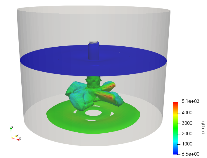
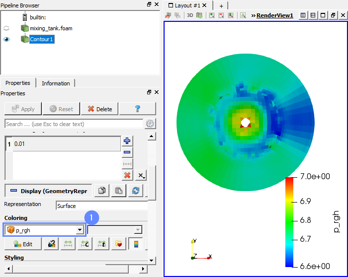
43. ParaView - Display Water Surface (II)
- Select contour coloring variable p_rgh
After change the coloring variable and opacity the contour will be shown in the 3D window. Note that the pressure on the water surface is constant.
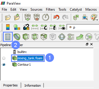
44. ParaView - Calculator (I)
- Select mixing_tank.foam
- Clcik Calculator
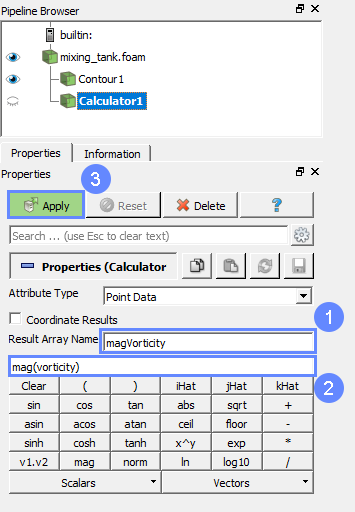
45. ParaView - Calculator (II)
- Change name to magVorticity
- Write the formula mag(vorticity)
- Click Apply
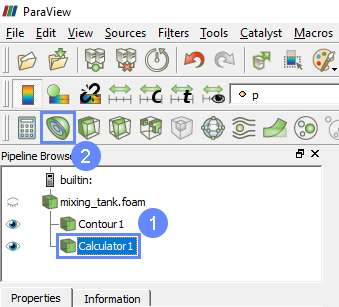
46. ParaView - Create Contour (I)
- Select Calculator 1
- Create Contour
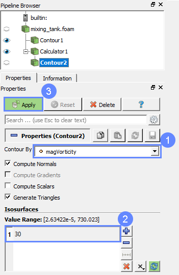
47. ParaView - Create Contour (II)
- Select magVorticity as a contour variable
- Set contour value to 30
- Click Apply
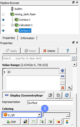
48. ParaView - Create Contour (III)
- Select contour coloring variable p_rgh
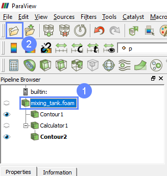
49. ParaView - Load geometry (I)
- Select mixing_tank.foam
- Click Open
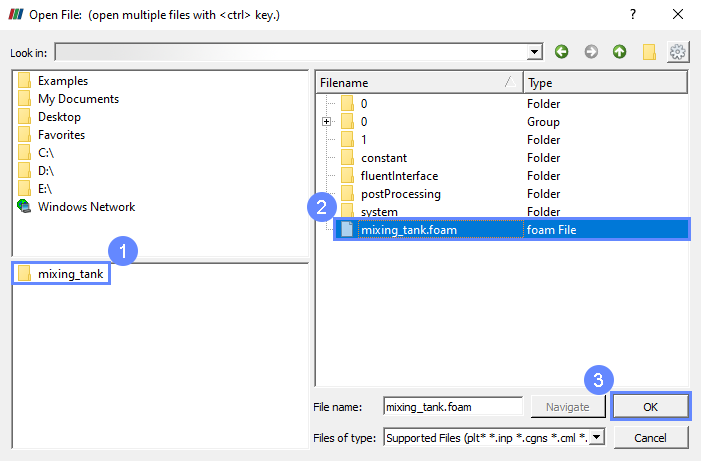
50. ParaView - Load geometry (II)
- Click mixing_tank
- Select mixing_tank.foam from file selection dialog
- Click OK
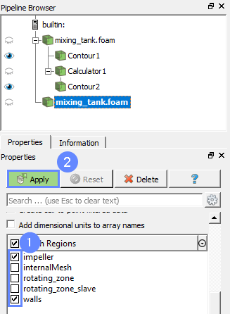
51. ParaView - Load geometry (III)
- Select impeller and walls zones to plot
- Click Apply
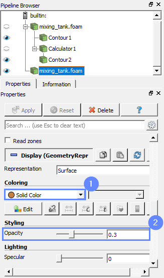
52. ParaView - Load geometry (IV)
- Set Coloring to Solid Color
- Set the opacity to 0.3
53. ParaView - Results
The results are displayed in the graphics window