3. Create Case
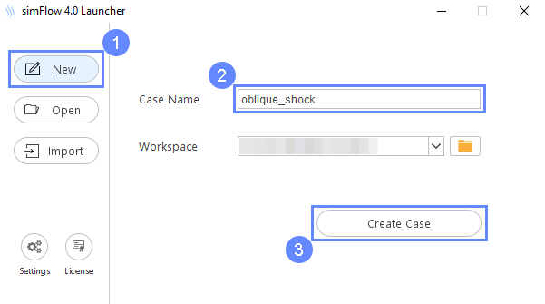
Open SimFlow and create a new case named oblique_shock
- Go to New panel
- Provide name oblique_shock
- Click Create Case
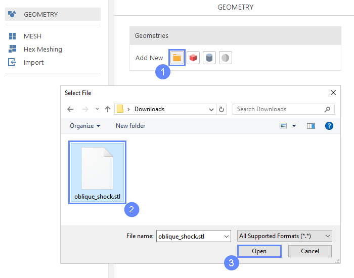
4. Import Geometry
Firstly, we need to Download GeometryOblique_shock and save it to the hard drive. Then:
- Click Import Geometry
- Select already downloaded geometry file oblique_shock.stl
- Click Open
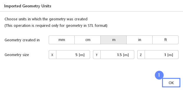
5. Imported Geometry Units
The STL format does not contain the unit information which are defined during the geometry export. If we do not know the exported unit, we can estimate it based on the total size of the model. It is displayed next to Geometry size label. In our case, the default unit meter is correct.
- To confirm default unit meter, press OK
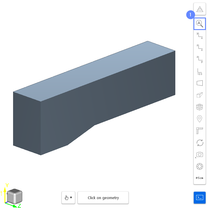
6. Geometry
After import, the tunnel geometry will be displayed in the graphics window.
- Click Fit View to zoom the geometry
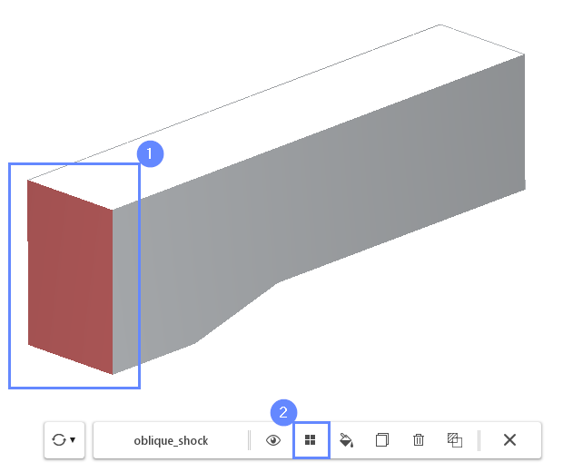
7. Creating Face Group - Inlet
We are dealing with an internal flow problem. The imported geometry determines the bounds of the fluid domain. To inform the program where different boundaries should be created, we will create appropriate face groups.
- Select the inlet face by holding CTRL key and clicking on the geometry face in a 3D view. The selection should be marked in red
- Click on the Face Group button in the graphics context toolbar
- Press Esc key to clear the selection
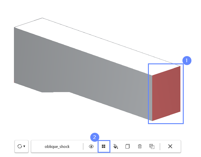
8. Creating Face Group - Outlet
Rotate the view in a way you will be able to see the second end of the tunnel.
- Select the outlet face by holding CTRL key and clicking on the geometry face
- Click on the Face Group button in the graphics context toolbar
- Press Esc key to clear the selection
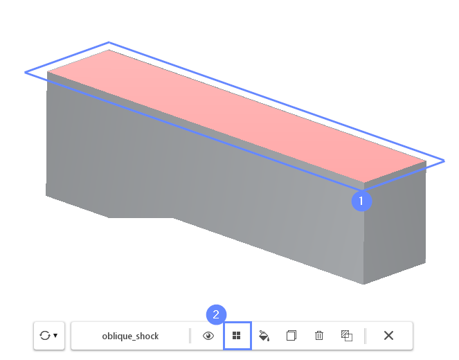
9. Creating Face Group - Top
Now, select the top face of the tunnel.
- Select the top face by holding CTRL key and clicking on the geometry face
- Click on the Face Group button in the graphics context toolbar
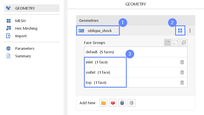
10. Rename Face Groups
In the Geometry Panel , under the oblique_shock geometry we can find four face groups. The first group, named default , contains all non-selected surfaces. These surfaces will form the bottom walls of the tunnel. The next two groups represent the inlet and outlet of the fluid domain respectively. The last one represents the top wall of the tunnel. We will rename these groups to make the resulting boundary names more readable.
- Select oblique_shock geometry
- Expand Geometry Faces
- Change face groups names accordingly (double click on its name and start editing)
group_1 \(\rightarrow\) inlet
group_2 \(\rightarrow\) outlet
group_3 \(\rightarrow\) top
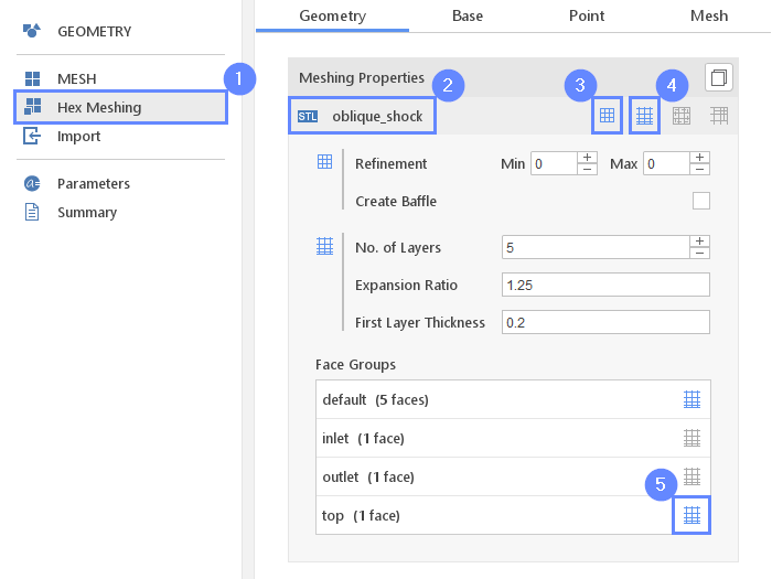
11. Meshing Parameters - Geometry
When geometry is ready we can move to the meshing step. We will define the boundary layer on the bottom and top wall of the tunnel.
- Go to Hex Meshing panel
- Select the oblique_shock component
- Enable Mesh Geometry
- Enable Create Boundary Layer Mesh
- Mark top face group to be inflated with a boundary layer
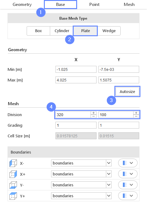
12. Base Mesh - Domain
In order to create a 2D mesh, we will use a Plate base mesh type.
- Go to Base tab
- Select Plate as a Base Mesh Type
- Click on Autosize
- Define the number of divisions
Division320100
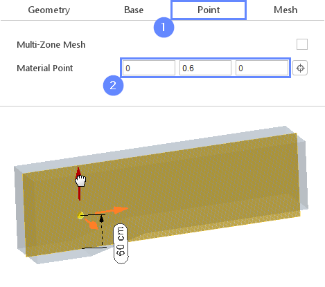
13. Solid Mesh - Material Point
Material Point tells the meshing algorithm on which side of the geometry the mesh is to be retained. Since we are considering flow inside the tunnel we need to place the material point inside the geometry.
- Go to Point tab
- Specify location inside the tunnel
Material Point00.60
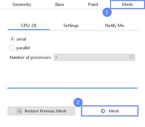
14. Start Meshing
Everything is now ready for meshing.
- Switch to Mesh tab
- Start the meshing process with Mesh button
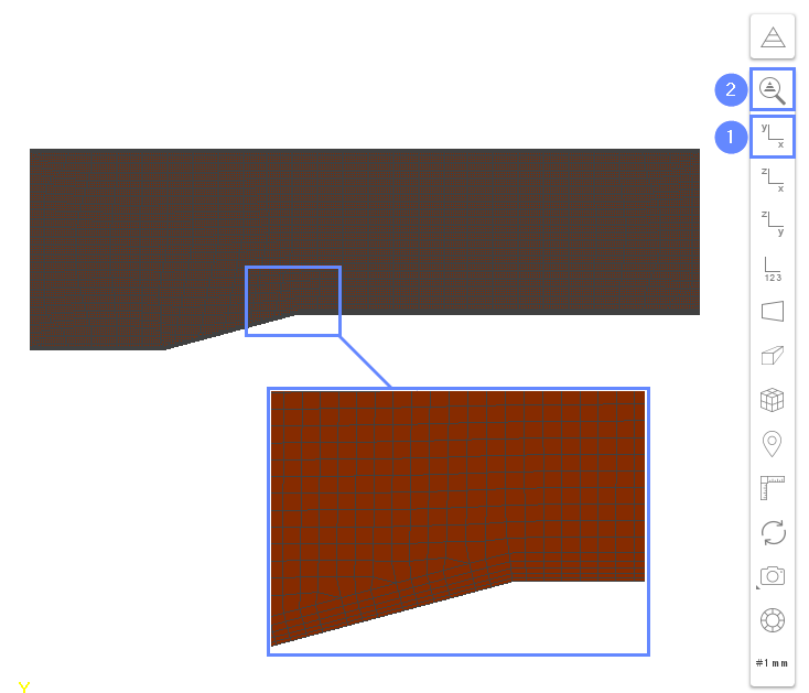
15. Mesh
After the meshing process is finished the mesh should appear on the screen.
- Set the XY orientation View XZ
- Click Fit View
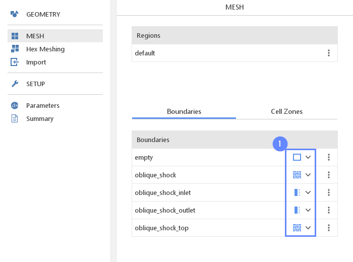
16. Boundaries
To be able to assign inlet and outlet boundary conditions we have to adjust the mesh boundary types.
- Define boundary types accordingly
empty Empty
oblique_shock Wall
oblique_shock_inlet Patch
oblique_shock_outlet Patch
oblique_shock_top Wall
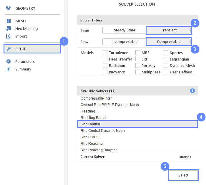
17. Select Solver
We want to analyze high-speed compressible flow inside the tunnel. For this purpose, we will use the Rho Central (rhoCentralFoam) solver.
- Go to SETUP panel
- Select Transient type
- Select Compressible flow filter
- Select Rho Central (rhoCentralFoam) solver
- Select solver
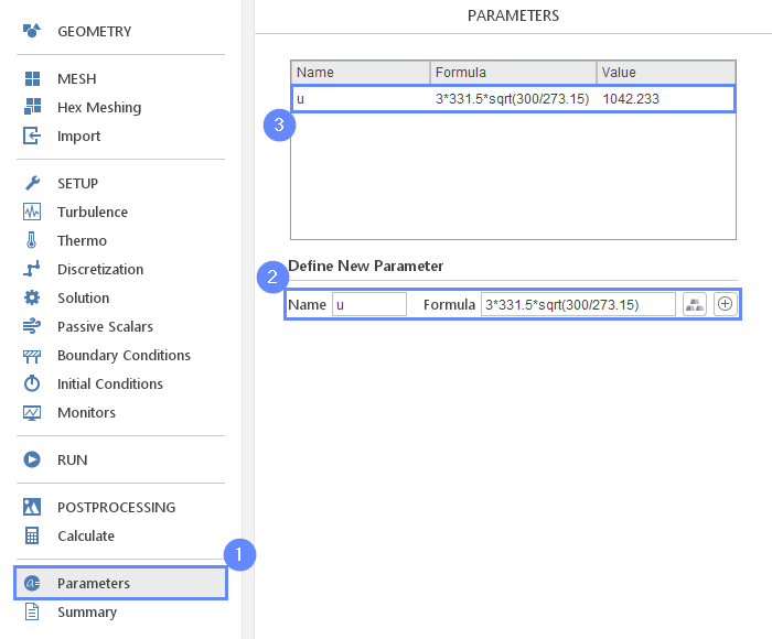
18. Parameters - Velocity
SimFlow allows users to create parameters that can be used instead of numbers. This allows to easily change a single property without the need to edit all inputs where a given property is used. In this tutorial, we will create a velocity parameter equal to 3 times the Mach number. The speed of sound for \(0^{\circ}C \; (273.15K)\) is \(331.5\; m/s\). To compute its value for temperature 300K we will use the following formula:
\(c_{air}=331.5 \cdot \sqrt{300/273.15}\)
- Go to Parameters panel
- Define the new parameter name and formula and press Enter
Nameu
Formula3*331.5*sqrt(300/273.15) - The newly created parameter will be shown in the parameters list.
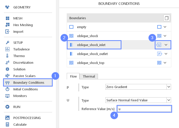
19. Boundary Conditions - Inlet - Flow
Now, we will define the inlet and outlet boundary conditions. At the inlet, we will set constant fluid velocity using parameter u .
- Go to Boundary Conditions panel
- Select oblique_shock_inlet boundary
- Set the Velocity Inlet character
- Set the inlet velocity
U Reference Value \({\sf [m/s]}\)u
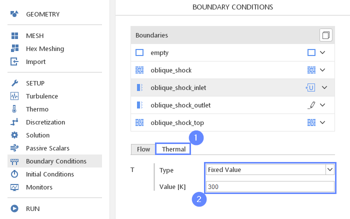
20. Boundary Conditions - Inlet - Thermal
- Switch to Thermal tab
- Set constant temperature at the inlet
T Type Fixed Value
T Value \({\sf [K]}\)300
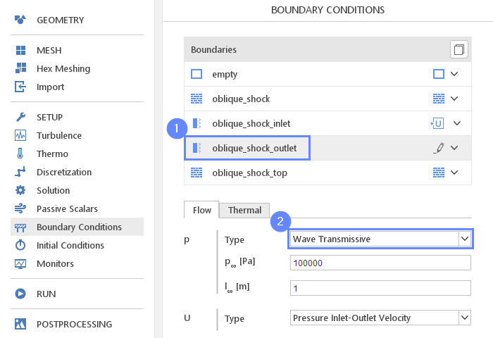
21. Boundary Conditions - Outlet
At the outlet, we are going to apply the Wave Transmissive boundary condition. This type allows the pressure waves to freely escape the domain and prevents reflecting them from the outlet boundary.
- Select oblique_shock_outlet
- Set the pressure type
p Type Wave Transmissive
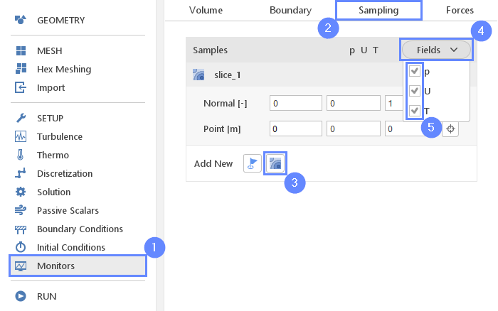
22. Monitors – Sampling
During calculation, we can observe intermediate results on a section plane. To add sampling data on a plane we need to define the plane and also select fields that will be sampled. Note that runtime post-processing can only be defined before starting calculations and can not be changed later on.
- Go to Monitors panel
- Switch to Sampling tab
- Select Create Slice
- Expand Fields list
- Select pressure p , velocity U and Temperature T
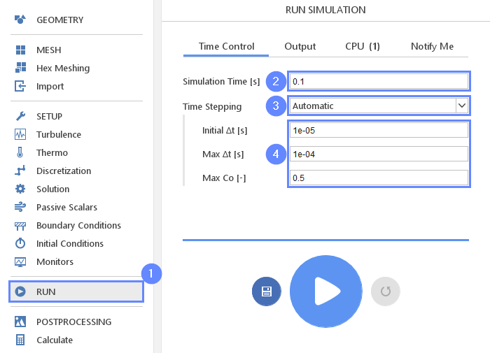
23. Run - Time Control
For any simulation, it is very convenient to let the solver automatically determine the proper time step value. To use this option we need to define time step constraints by providing the initial time step (adjusted by the solver during computations), maximal time step value and the Courant number.
- Go to RUN panel
- Set the Simulation Time [s] to 0.1
- Change Time Stepping to Automatic
- Set initial time step, maximum time step and the Courant number accordingly
Initial \(\Delta t\) \({\sf [s]}\)1e-05
(solver will start computation with this value and adjust it in the next iterations)
Max \(\Delta t\) \({\sf [s]}\)1e-04
Max Co \({\sf [-]}\)0.5
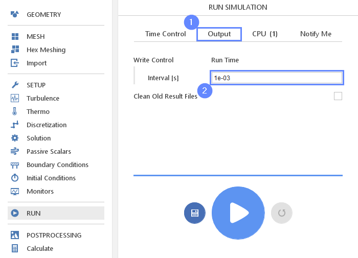
24. Run - Output
We can control how often results should be saved on the hard drive. Only this data will be available for postprocessing.
- Switch to Output tab
- Set the Interval [s] to 1e-03
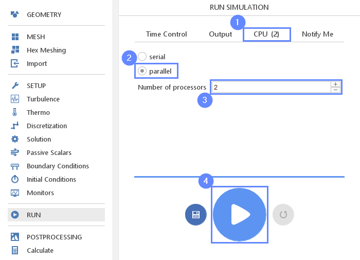
25. Run - CPU
To speed up calculation process increase the number of CPUs basing on your PC capability. We recommend using 4 cores for this tutorial. If you are using a free version you can use the contact form to Request 30-day Trial
Estimated computation time for the free version (2 processors): 20 minutes
- Switch to CPU tab
- Change the solver to parallel
- Define the number of processors
- Click Run Simulation button
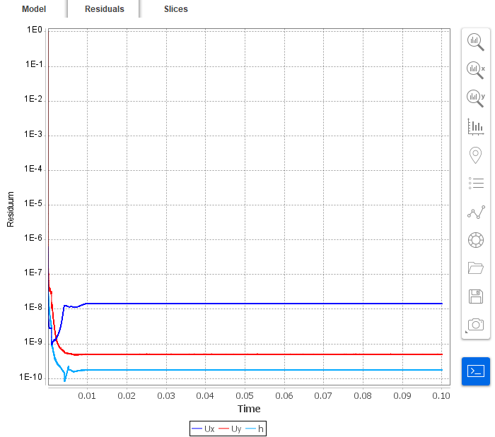
26. Residuals
When the calculation is finished you should see a similar residual plot.
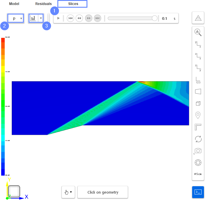
27. Slice - Velocity Field
During computation Slices tab will appear next to the Residuals. Under this tab, we can preview results on the section plane.
- Change tab to Slices
- Select the pressure p
- Click Adjust range to data
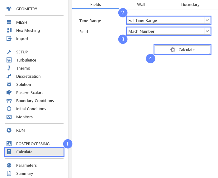
28. Calculate Vorticity
The Mach number is not being computed by default during solver computations. In order to visualize it, we will compute the Mach number using the existing data.
- Go to Calculate panel
- Set the Time Rnge to Full Time Range
- Set the Field to Mach Number
- Click on Calculate
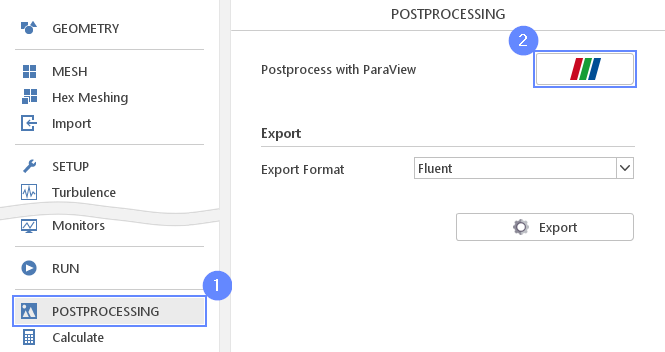
29. Postprocessing – ParaView
Start ParaView to visualize the shock wave.
- Go to POSTPROCESSING panel
- Click on Run ParaView
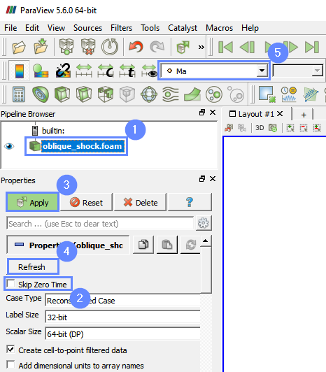
30. ParaView - Load Results
Load the results into the program.
- Select oblique_shock
- Uncheck Skip Zero Time
- Click Apply to load results into ParaView
- Click Refresh
- Select Mach number Ma from the list
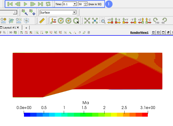
31. ParaView - Vorticity
The Mach number contour plot will be displayed in the graphic window.
- Play with animation buttons to track the flow history
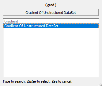
32. ParaView - Pressure Gradient (I)
In order to see shock waves more clearly we will display gradients of pressure p which will indicate the discontinuity region.
- While holding the Ctrl key push the Spacebar
- Start typing Gradient of Unstructured DataSet and press Enter to select this command
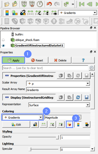
33. ParaView - Pressure Gradient (II)
Now we will display the magnitude of the pressure gradient in the 3d view. We can adjust the coloring scheme to see the shock waves more clearly.
- Click Apply to display Pressure Gradient
- Select Gradients from the Coloring list
- Click Choose preset
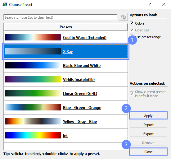
34. ParaView - Coloring
We would like to have similar plots to the Schlieren photography which is often used in experiments to visualize density variation. For this purpose we will use X Ray preset.
- Select X Ray preset.
- Apply changes
- Close window
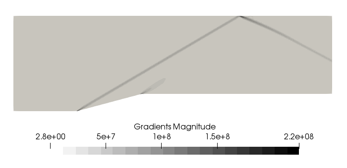
35. Paraview - Shock Wave - Results
Shock waves can be identified at the locations of the largest pressure gradient, which corresponds to the dark color in the image. The shock wave angle depends on the wedge angle and Mach Number.
In our case, the shock wave angle equals 31 degrees and is very close to the theoretical value. The analytical solution of this problem is well known and for instance, it can be found in:
Anderson J. Modern Compressible Flow: With Historical Perspective. McGraw-Hill Series in Aeronautical and Aerospace Engineering. McGraw-Hill, 2004. ISBN 9780071241366