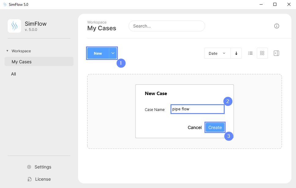
3. Create Case
Open SimFlow and create a new case named pipe flow
- Click New
- Provide name pipe flow
- Click Create to open a new case
4. Create Geometry - Cylinder 1
To build a "Pipe" geometry for the simulation, we will make use of SimFlow’s basic geometry module. This module allows for creating and editing of primitive geometries (box, cylinder, and sphere).
SimFlow also supports importing complex geometries in well known formats such as STEP, STL, IGES, and others. However, in this case, we will use a simple pipe geometry.
For this operation, we will need to create two cylinders, which we will unite in further steps into a pipe. Our initial step will involve adding the first cylinder.
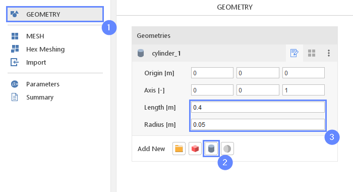
- Go to Geometry panel
- Select Create Cylinder
- Set the cylinder dimensions:
Length \({\sf [m]}\)0.4
Radius \({\sf [m]}\)0.05
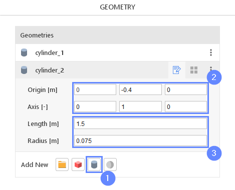
5. Create Geometry - Cylinder 2
In this step we will create second cylinder.
- Select Create Cylinder
- Set the origin and axis:
Origin \({\sf [m]}\)0-0.40
Axis \({\sf [-]}\)010 - Set the cylinder dimensions:
Length \({\sf [m]}\)1.5
Radius \({\sf [m]}\)0.075
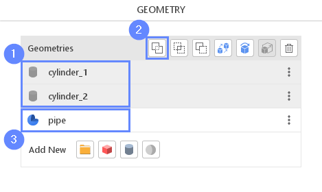
6. Unite Geometries
In this step we will create a pipe geometry by joining two cylinders created in prior steps. For this task we will use an unite tool. This is a geometric boolean operation that will result in a single solid geometry.
- Select both cylinder with CTRL key pressed
- Click Unite Geometries
- New geometry will be listed below the cylinders. Double click on its name and change it from unite to pipe
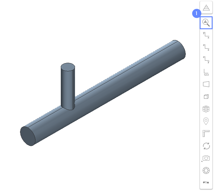
7. Geometry - Pipe
The resulting geometry will be displayed in the graphics window.
- Click Fit View to zoom in the geometry
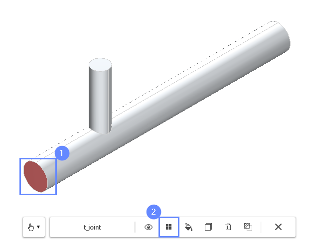
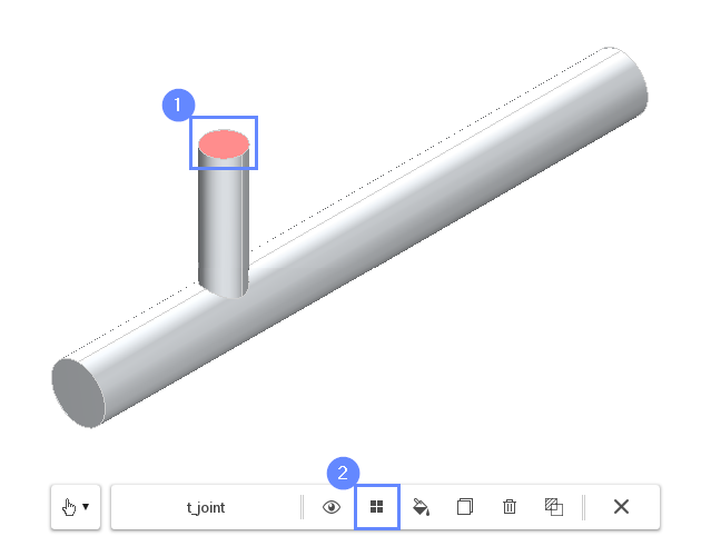
8. Creating Face Group - Inlet 1
In this simulation, we are dealing with an internal flow problem. The imported geometry determines the bounds of the fluid domain. To inform the program where the boundaries of the inlet and outlet mesh should be created, we will use the Face Groups.
Face Group is a set of faces that should be distinguished within a geometry. When the geometry containing the face group is used for meshing, an additional boundary is created. The boundary represents the respective face group and inherits its name.
- Select the first inlet face by holding CTRL key and clicking on the geometry face in a 3D view. The selection should be marked in red
- Click on the Face Group button in the graphics context toolbar
- Press Esc or click the X button to exit selection mode
9. Creating Face Group - Inlet 2
In this step we will create a face group for the second inlet.
- Select the second inlet. Press CTRL key and click on the face as shown on the slide below
- Click on the Face Group button in the graphics toolbar
- Press Esc or click the X button to exit selection mode
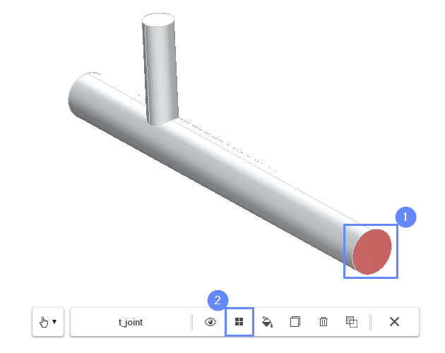
10. Creating Face Group - Outlet
In order to choose the outlet, we need to rotate the view so that the other end of the geometry becomes visible.
- Select the outlet face. Press CTRL key and click on the face
- Click on the Face Group button in the context toolbar
- Press Esc or click the X button to exit selection mode
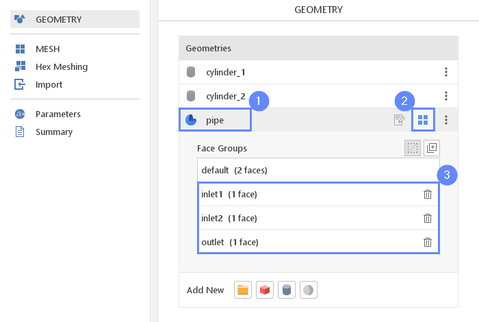
11. Rename Face Groups
In the Geometry Panel we can find four Face Groups under the pipe geometry. The first group, named default, contains all non-selected surfaces. These surfaces will become the pipe walls.
The three additional groups represent the inlets and the outlet of the fluid domain. We will rename those groups to make the resulting boundary names more readable.
- Select pipe geometry
- Expand Geometry Faces
- Change face groups names accordingly (double-click on a group name to start editing)
group_1 \(\rightarrow\) inlet1
group_2 \(\rightarrow\) inlet2
group_3 \(\rightarrow\) outlet
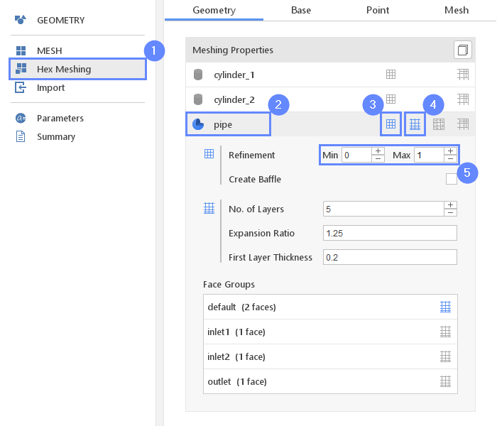
12. Meshing Parameters - Pipe
In order to create the mesh, we need to specify the meshing options used for a given geometry. For the pipe, we will add the boundary layer and refine the mesh near edges by level 1.
- Go to Hex Meshing panel
- Select the pipe component
- Enable Mesh Geometry
- Enable Create Boundary Layer Mesh
- Set surface Refinement to Min 0 Max 1
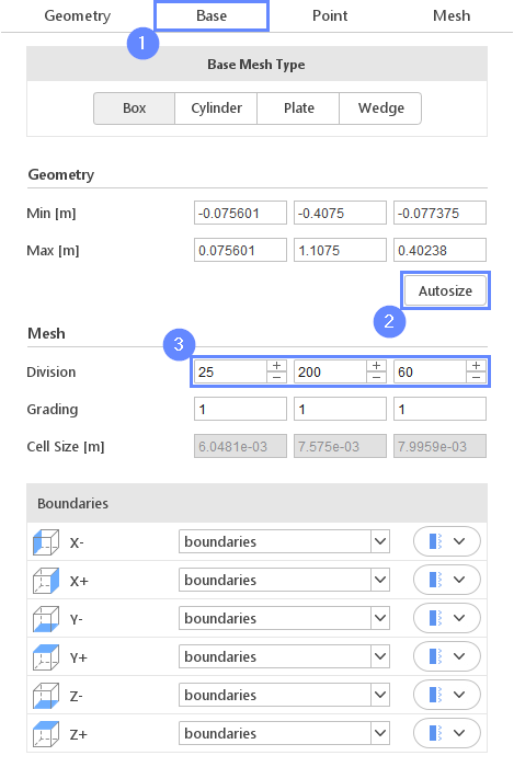
13. Base Mesh - Domain
For the base mesh, we will use a box geometry. As we would like to create the mesh inside the pipe geometry, we need to make the box size a little bigger than the pipe.
- Go to Base tab
- Click on Autosize to adopt box to visible geometries
- Define the number of divisions
Division2520060
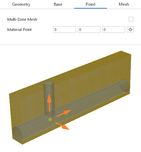
14. Material Point
Material Point tells the meshing algorithm on which side of the geometry the mesh is to be retained.
Since we are considering flow inside the pipe we need to place the material point inside the geometry. In this case, we do not need to modify the coordinates of the material point, since the default location is already inside the pipe.
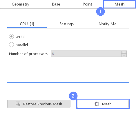
15. Start Meshing
In this step we will initiate the meshing process.
In the meshing panel you may indicate how many CPUs would you like to use for this process. Please note that if you are using SimFlow free version you may only use serial meshing, and you may not create meshes larger than 200'000 nodes.
If you would like to test full version Request 30-day Trial
- Switch to Mesh tab
- Start the meshing process with Mesh button
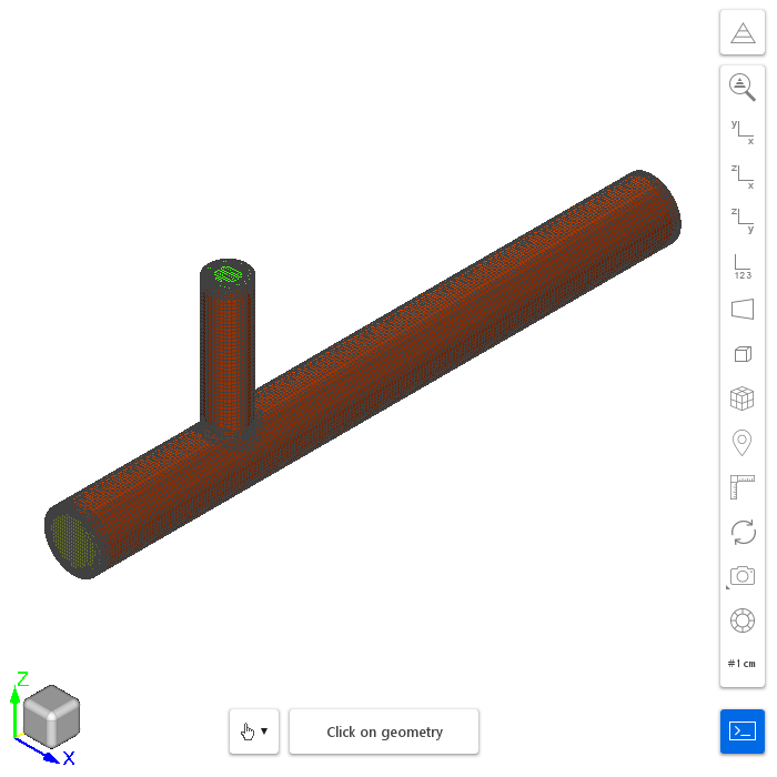
16. Mesh
After the meshing process is finished the mesh should appear on the screen.
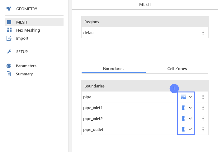
17. Boundaries
To be able to assign inlet and outlet boundary conditions we have to assign the proper boundary types.
- Define boundary types accordingly
pipe wall
pipe_inlet1 patch
pipe_inlet2 patch
pipe_outlet patch
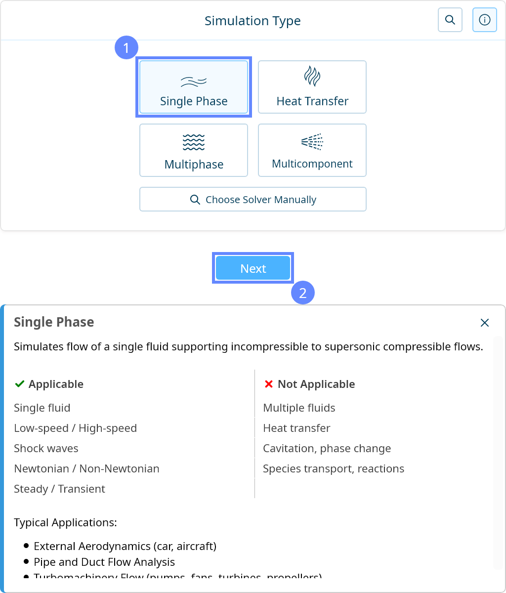
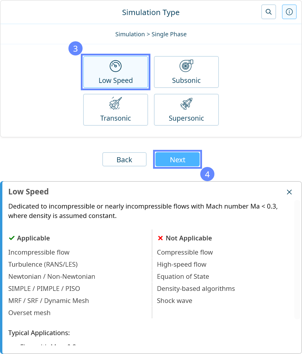
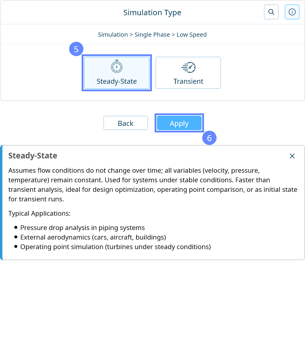
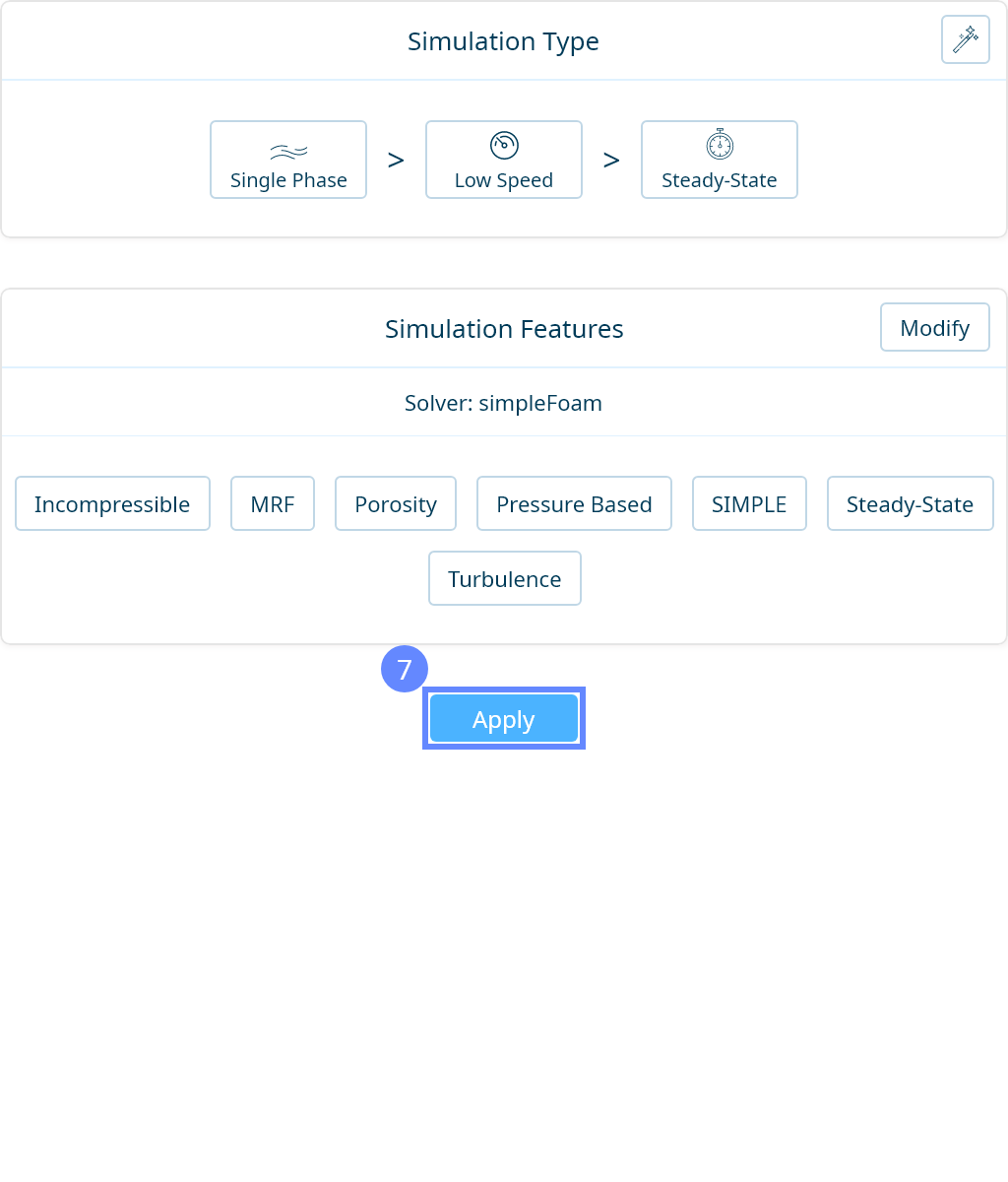
18. Simulation Type
We want to analyze the water flow through a pipeline. For this purpose, we will use a single-phase, steady-state simulation of incompressible turbulent flow.

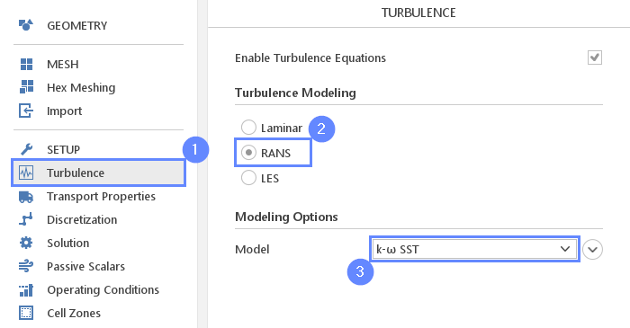
19. Turbulence
We are going to use the standard \(k{-}\omega \; SST\) model to resolve turbulence.
- Go to Turbulence panel
- Select RANS modeling
- Select \(k{-}\omega \; SST\) model
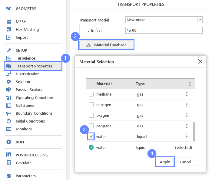
20. Transport Properties - Water
As a fluid material, we will use water.
- Go to Transport Properties panel
- Open Material Database
- Pick up water from the list
- Click Apply
Selecting material from the Material Database will fill all inputs in the Transport Properties panel. We are still able to overwrite these values at any time.
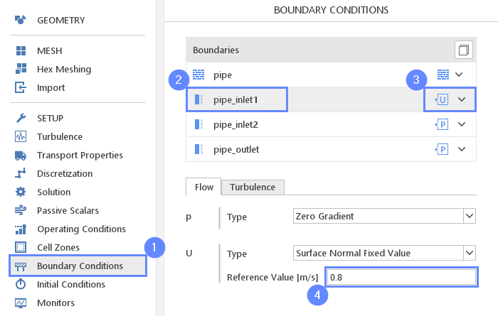
21. Boundary Conditions - Inlet 1
Now, we will define the inlet and outlet boundary conditions. At the first inlet, we will set constant water velocity.
- Go to Boundary Conditions panel
- Select pipe_inlet1 boundary
- Set the Velocity Inlet character
- Set the inlet velocity
U Reference Value \({\sf [m/s]}\)0.8
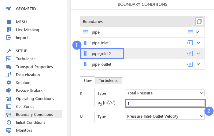
22. Boundary Conditions - Inlet 2
The second inlet will be defined using pressure inlet condition. For the pressure value, we will use 1 [kPa].
Note, for the incompressible solver, we operate using kinematic properties. And thus instead of using dynamic pressure, we are going to set a value divided by reference density – kinematic pressure \(m^2/s^2\).
- Select pipe_inlet2
- Set the total pressure value
\(p_0\) \({\sf [m^2 / s^2]}\)1
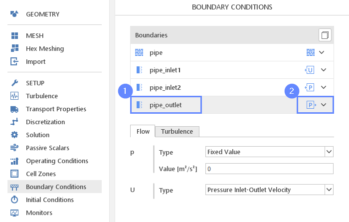
23. Boundary Conditions - Outlet
At the outlet, we will apply pressure outlet character. The pressure value we will leave default 0. For the incompressible flow, pressure is always relative and we can add any constant (1 atm for example) after computation.
- Select pipe_outlet
- Set the Pressure Outlet character
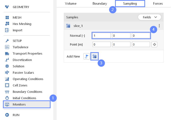
24. Monitors – Sampling (I)
During calculation, we can observe intermediate results on a section plane. To sample data on a plane we need to define the plane and also select fields that will be sampled. Note, runtime post-processing can only be configured before starting calculations and can not be changed later on.
- Go to Monitors panel
- Switch to Sampling tab
- Select Create Slice
- Set slice plane normal vector
Normal \({\sf [-]}\)100
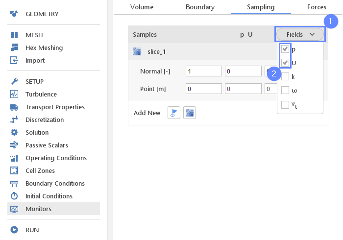
25. Monitors – Sampling (II)
Additionally, we need to specify the variables to be sampled.
- Expand Fields list
- Select pressure p and velocity U
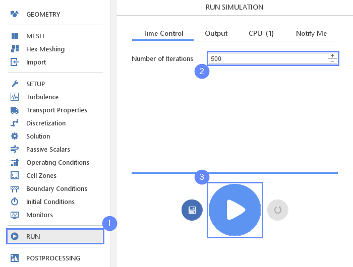
26. Run - Time Control
Finally, we can start our computation.
Estimated computation time for single-core: 5 minutes
- Go to RUN panel
- Set the maximum Number of Iteration to 500
- Click Run Simulation button
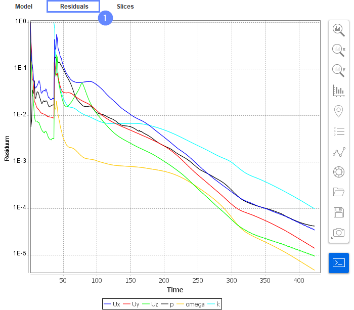
27. Residuals
When the calculation is finished we should see a similar residual plot. All the residual values have reached \(10^{-4}\) and the solver has automatically stopped the calculation. The residuals are the measure of how results change between iteration. Reaching a very low value indicates that we have found a steady-state solution and results do not change regardless of further computations.
- Go to Residuals tab
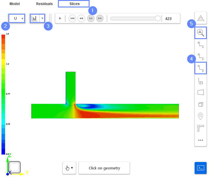
28. Slice - Velocity Field
Slices tab appears next to the Residuals. Under this tab, we can preview results on the defined section plane.
- Change tab to Slices
- Select the velocity U
- Click Adjust range to data
- Set the YZ orientation View YZ
- Click Fit View
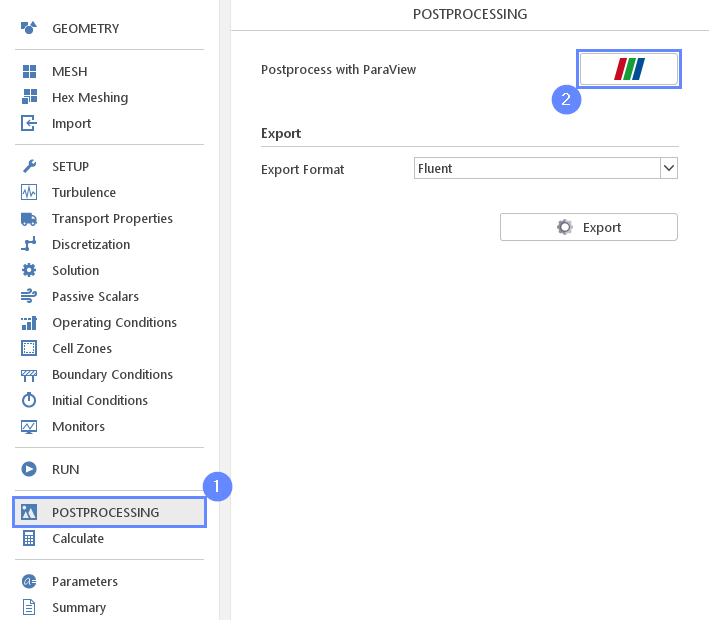
29. Start Postprocessing with ParaView
To access more advanced postprocessing functions, use the integrated ParaView software.
- Go to Postprocessing panel
- Run ParaView
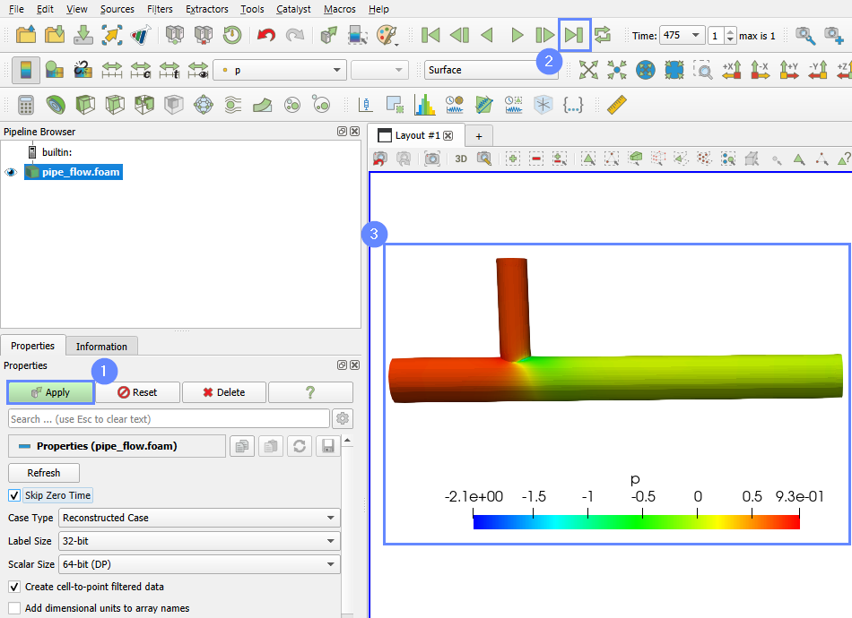
30. ParaView - Load Results
A new ParaView window should open. Load results into the ParaView. Be aware that in a steady-state simulation, SimFlow saves only the last two iterations by default. View the last one to see the final solution.
- Click Apply to load results into ParaView
- Display the results from the last frame
- After loading results, they will be shown in the 3D graphic window
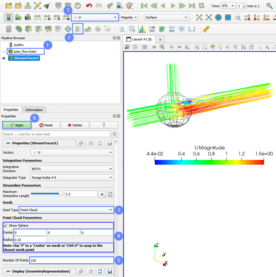
31. ParaView - Display Streamlines (I)
Advanced postprocessing features give us a possibility to display i.e., streamlines. To do that, follow these steps:
- Make sure the pope_flow.foam case is selected and highlighted in blue
- Select Stream Tracer from the top menu
- Change Seed Type to Point Cloud
- Type the center coordinate and radius of the sphere:
Center000
Radius0.15 - Increase the number of points to 150
- Click Apply
- Select the velocity U from the list
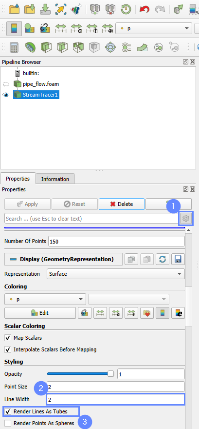
32. ParaView - Display Streamlines (II)
To enhance visibility, we can render the streamlines.
- Expand the Toggle advanced properties
- Scroll down to a Styling section and increase Line Width to 2
- Mark Render Lines As Tubes option
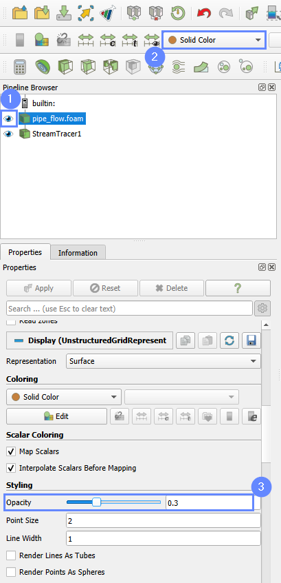
33. ParaView - Display Transparent Geometry
We can additionally display the transparent geometry to observe how the streamlines are distributed in relation to it.
- Click on the eye next to the pipe_flow.foam base case to display it
- Select the Solid Color from the list
- Set the Opacity to 0.3
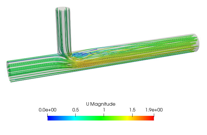
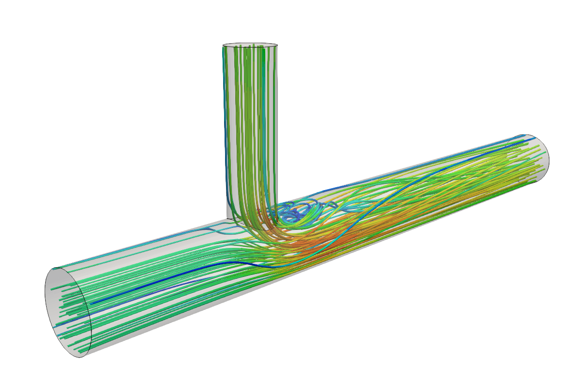
34. ParaView - Streamline Results
The final results contain the transparent geometry and streamlines colored by the velocity.