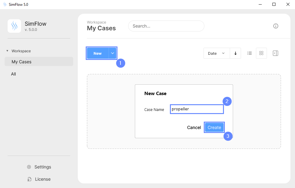
3. Create Case
Open SimFlow and create a new case named propeller
- Click New
- Provide name propeller
- Click Create to open a new case
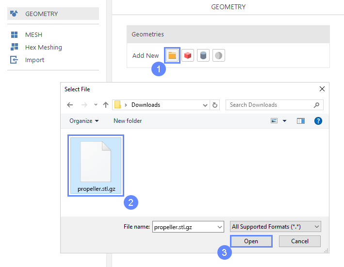
4. Import Geometry - Propeller
After creating case Download GeometryPropeller
- Click Import Geometry
- Select geometry file propeller.stl.gz
- Click Open
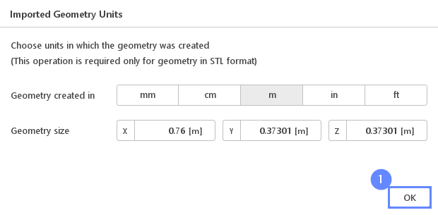
5. Imported Geometry Units
The STL format does not contain the unit information which are defined during the geometry export. Therefore, you must manually specify the correct unit after import. If we do not know the exported unit, we can estimate it based on the total size of the model. It is displayed next to Geometry size label. In our case, the default unit meter is correct.
- To confirm default unit meter, press OK
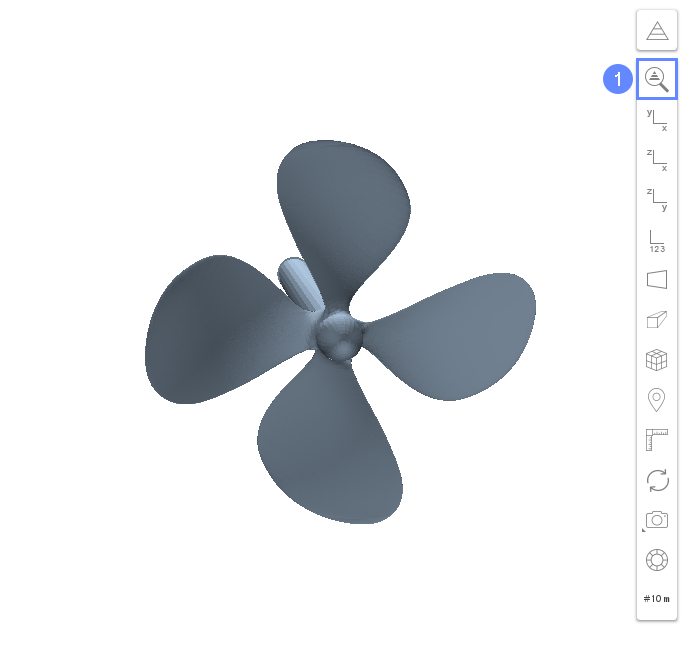
6. Propeller Geometry
After importing geometry, it will appear in the 3D window.
- Click Fit View to zoom the geometry
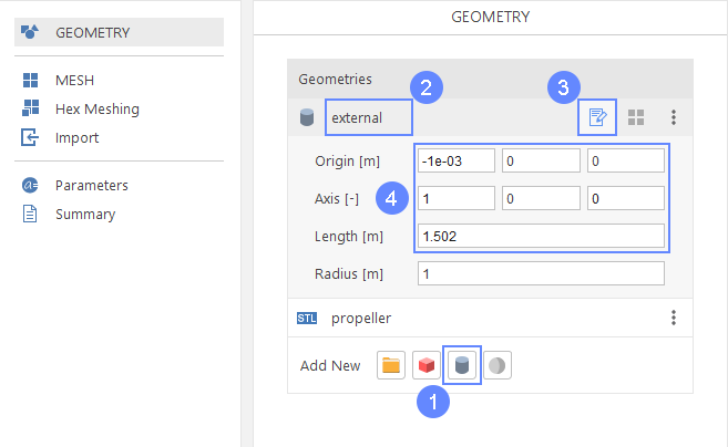
7. Domain Boundary
We need to create a cylindrical boundary for the domain. For this purpose, we will create a cylindrical geometry for later use in the meshing process.
- Click Create Cylinder
- Rename cylinder_1 to external
(double click on the name to rename it, press enter to apply) - Click Properties button if properties panel is not displayed
- Set origin, axis, and length of the cylinder accordingly
Origin \({\sf [m]}\)-1e-0300
Axis \({\sf [-]}\)100
Length \({\sf [m]}\)1.502
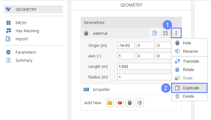
8. Refinement Area (I)
To better resolve the flow near the propeller, we will create an area with a higher mesh resolution. To do this, we will create a new geometry by copying settings from external geometry.
- Click Options of the external geometry
- Select Duplicate option
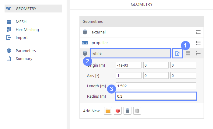
9. Refinement Area (II)
- Click Properties if they are not displayed
- Rename external_1 to refine
- Set radius of the refinement geometry
Radius \({\sf [m]}\)0.3
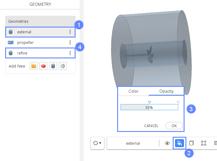
10. Display Geometries
In order to see all geometries, we will decrease the opacity of the external and refine.
- Select external
- Click Display Properties
- Adjust Opacity to 50%
- Adjust opacity to 50% for refine geometry by repeating previous steps
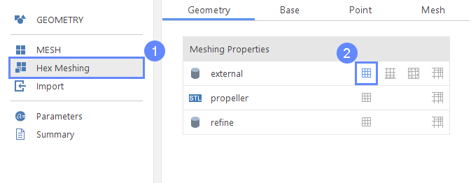
11. Meshing Parameters - External
Once the geometry is prepared, we can define the meshing properties. Meshing will be enabled for the external geometry, as it serves as the outer boundary of the analysis domain.
- Go to Hex Meshing panel
- Enable Mesh Geometry on external geometry
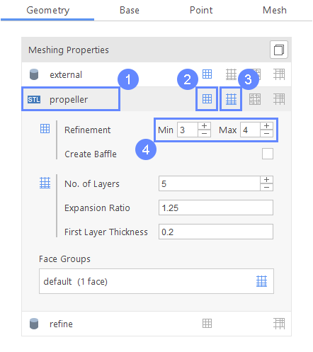
12. Meshing Parameters - Propeller
To better capture the flow around the blades, we refine the mesh near the propeller geometry by defining minimum and maximum refinement levels and applying a boundary layer mesh.
- Select propeller geometry
- Enable Mesh Geometry
- Enable Create Boundary Layer Mesh
- Set Refinement to Min 3 Max 4
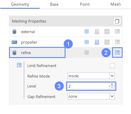
13. Meshing Parameters - Refine
We apply mesh refinement in the region influenced by the propeller-induced flow.
- Select refine geometry
- Enable Mesh Geometry
- Set refinement Level to 2
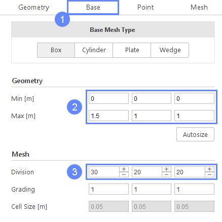
14. Base Mesh
We want to create a mesh of only one blade of the propeller. For this purpose, we will create a base mesh covering only one-fourth of the geometry.
- Go to the Base tab
- Define base mesh minimum and maximum extend
Min \({\sf [m]}\)000
Max \({\sf [m]}\)1.511 - Define Division along each axis
Division302020
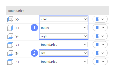
15. Base Mesh Boundaries
- 2 Define boundary names accordingly
X- inlet
X+ outlet
Y- right
Z- left
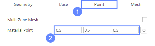
16. Material Point
The material point indicates which side of the geometry the mesh will be retained on. Since we are simulating airflow around the propeller, the material point must be placed outside the propeller geometry.
- Go to Point tab
- Set location of the material point
Material Point0.50.50.5
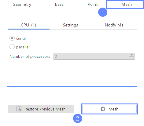
17. Start Meshing Process
In this step, we will initiate the meshing process.
In the meshing panel, you may indicate how many CPUs would you like to use for this process. Please note that if you are using SimFlow free version, you may only use serial meshing, and you may not create meshes larger than 200'000 nodes.
If you would like to test full version Request 30-day Trial
- Go to Mesh tab
- Start the meshing process with Mesh button
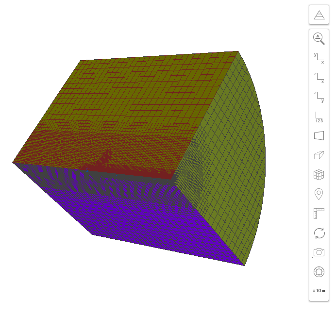
18. Mesh
After the meshing process is finished, the mesh should appear on the screen.
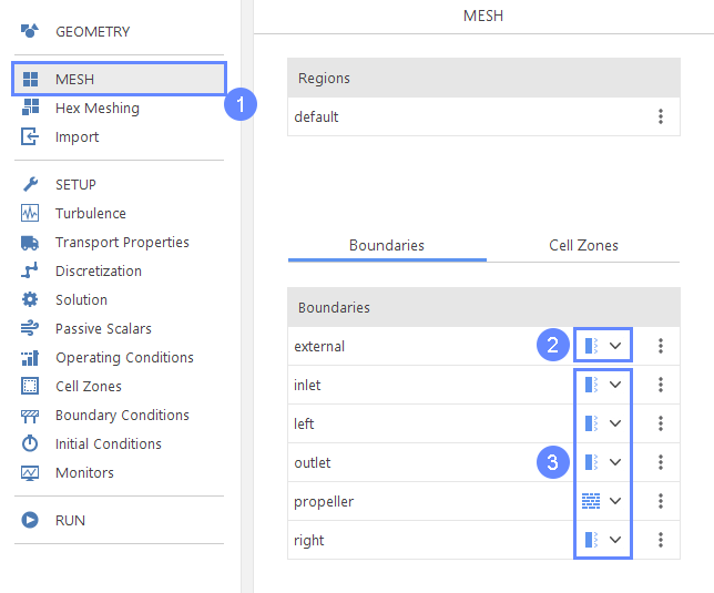
19. Boundary Types
After creating the mesh, we have to set proper boundary types.
- Go to Mesh panel
- Change the boundary type of the external geometry to patch
- Ensure that the remaining boundary types are selected appropriately
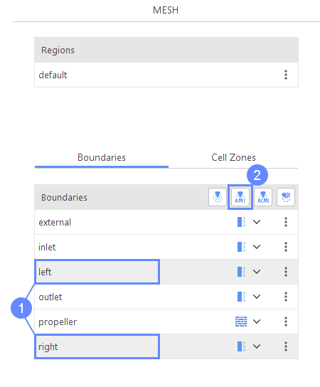
20. Boundary Interface (I)
As we will be simulating only one blade of the propeller, we have to create a boundary interface to make the model periodic.
- Hold CTRL key and select left and right boundary
- Click Create Arbitrary Interface between left and right boundary
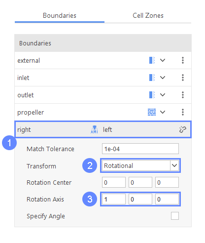
21. Boundary Interface (II)
- Expand the interface properties
- Change Transform type to Rotational
- Define Rotation Axis
Rotation Axis100
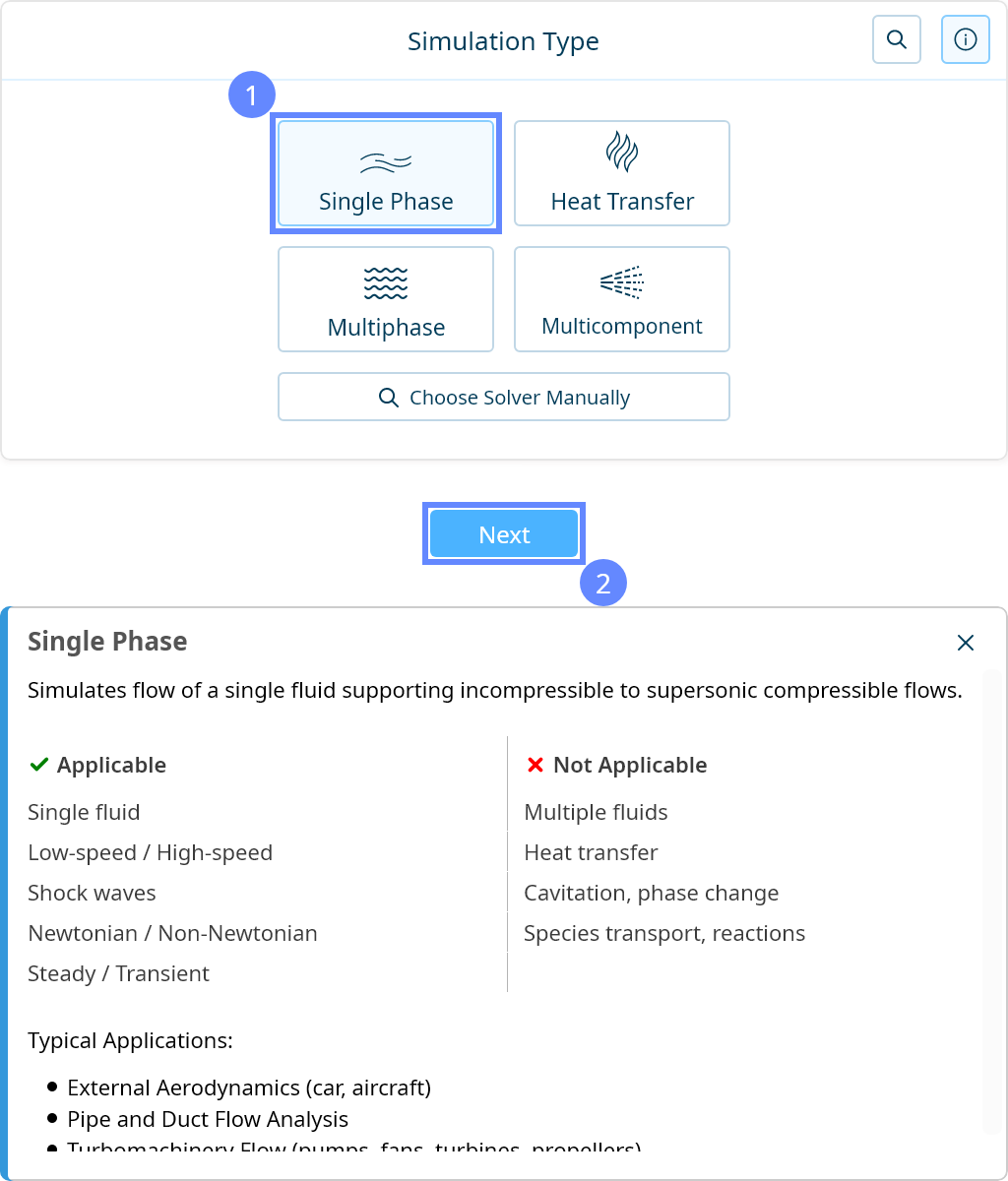
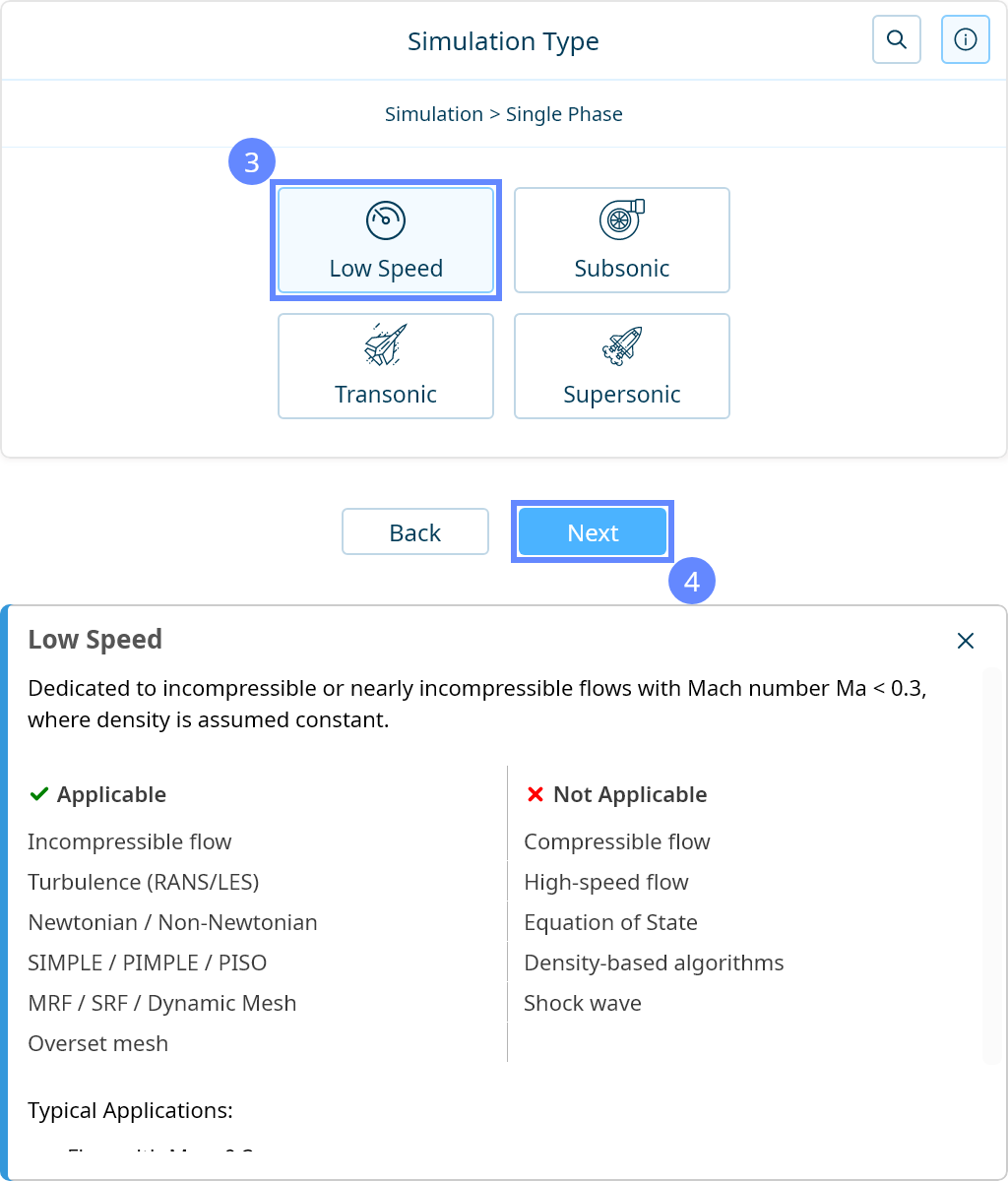
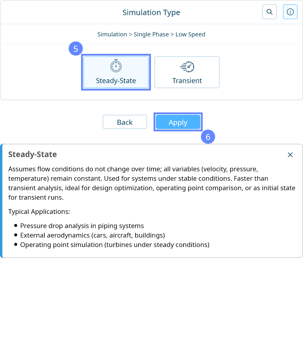
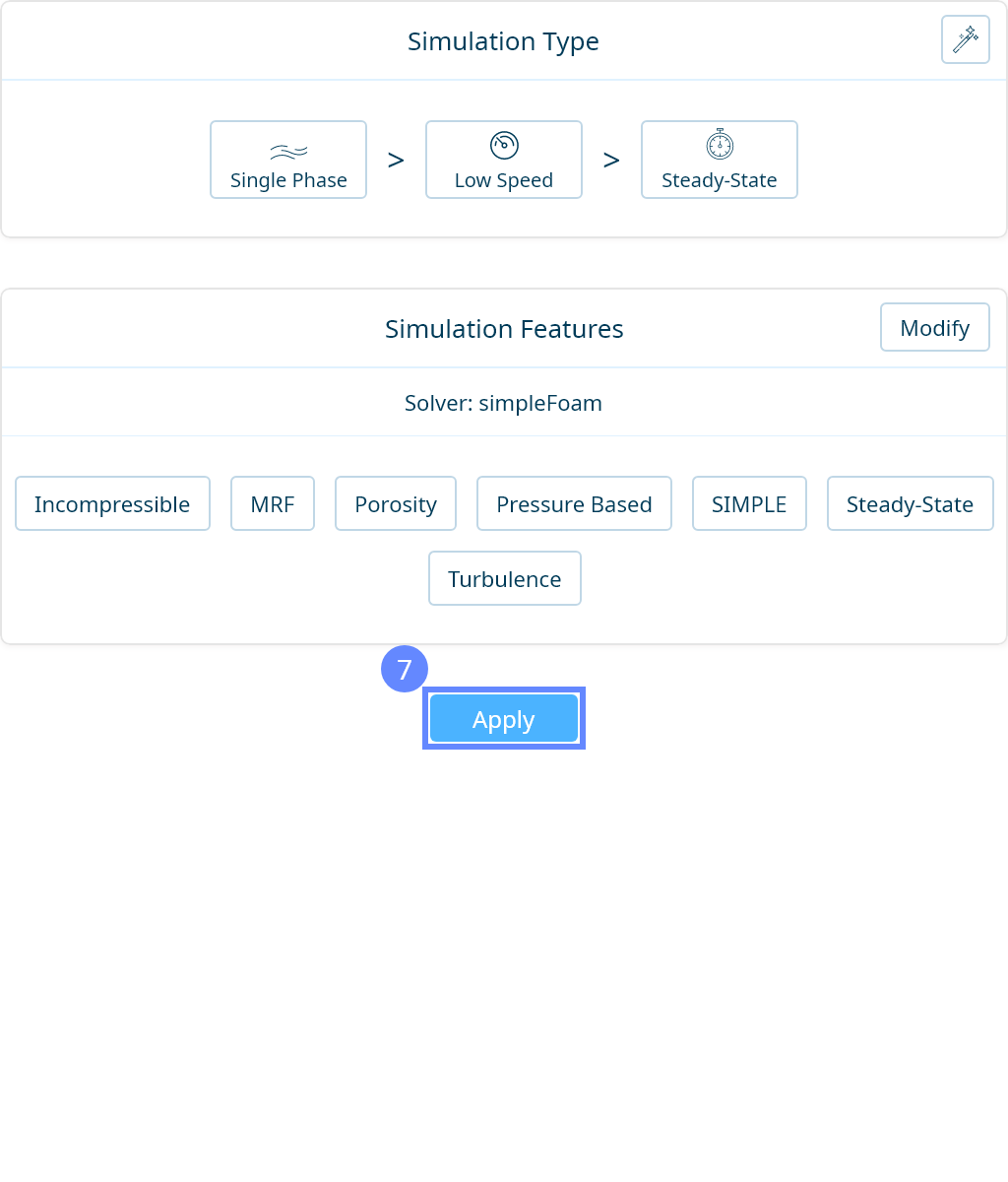
22. Simulation Type
We want to analyze the water flow around a marine propeller. For this purpose, we will use a single-phase, steady-state simulation of incompressible turbulent flow with Multiple Reference Frame (MRF).

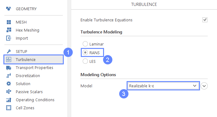
23. Turbulence Model
For the purpose of this tutorial we will simulate the turbulence phenomenon using \(Realizable \; k{-} \varepsilon\) model.
- Go to Turbulence panel
- Select RANS modeling
- Select \(Realizable \; k{-} \varepsilon\) turbulence model
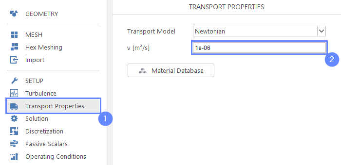
24. Water Properties
As a fluid material, we will use water.
- Go to Transport Properties panel
- Open Material Database
- Pick up water from the list
- Click Apply
Selecting material from the Material Database will fill all inputs in the Transport Properties panel. We are still able to overwrite these values at any time.
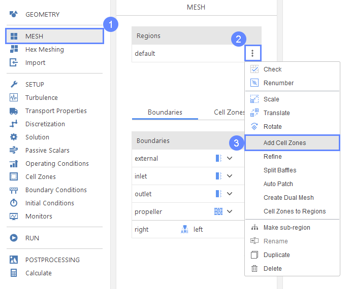
25. Cell Zones for MRF (I)
To be able to model propeller rotation, we will take advantage of a rotating reference frame. This technique will allow modeling the propeller rotation without a need to rotate the mesh. The rotating reference frame can only be applied to a sub-region of the mesh defined by a cell zone object (a list of mesh cells). Therefore, we will first create a cell zone.
- Go to Mesh panel
- Expand list of options form the default region
- Select Add Cell Zones from the menu
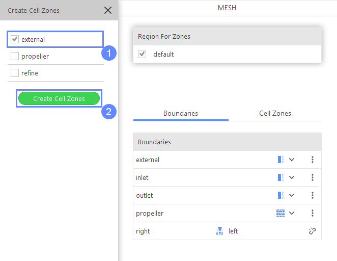
26. Cell Zones for MRF (II)
For the purpose of this tutorial, we will use the whole mesh as the rotating zone. To do this, we need to create the cell zone inside the external geometry.
- Select external geometry
- Click Create Cell Zones
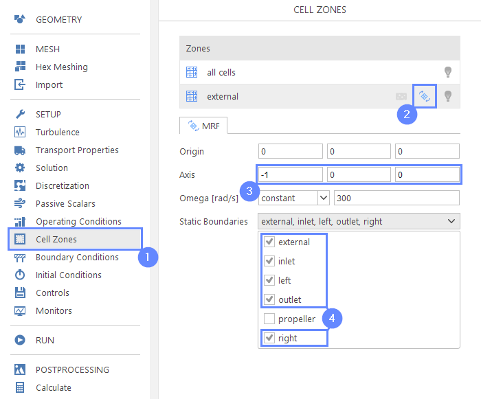
27. Rotating Reference Frame
The rotating reference frame should be aligned with the negative X-axis, and all boundaries except the propeller should be treated as stationary.
- Go to Cell Zones panel
- Enable Rotating Reference Frame for external zone
- Define Axis of the propeller
Axis-100 - Select boundaries that will not be defined in the rotating frame of reference
Static Boundaries:
external
inlet
left
outlet
right
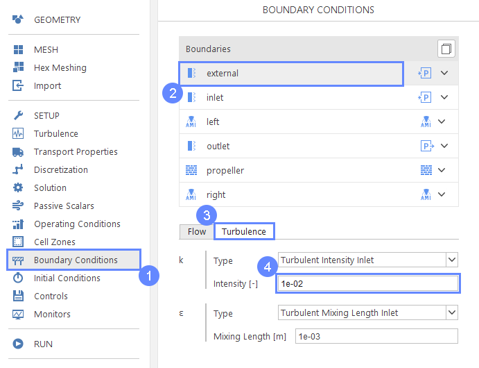
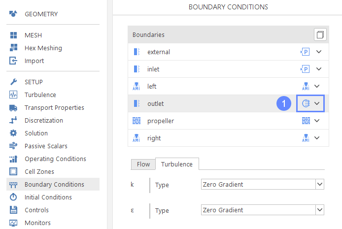
28. Boundary Conditions - External (Turbulence)
Next, we define the boundary conditions. Since the flow is driven by the rotating propeller, the external boundary should be set to a pressure inlet. Adjust only the turbulent intensity as follows.
- Go to Boundary Conditions panel
- Select external boundary
- Select Turbulence tab
- Set Turbulence Intensity to 1e-02
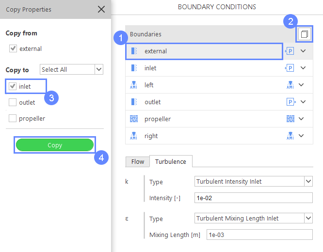
29. Boundary Conditions - Inlet
We will use the same boundary conditions for inlet and external boundaries, to achieve this we can copy settings from the external boundary to inlet.
- Make sure you have selected the external boundary
- Click Copy Boundary Conditions
- Select inlet boundary
- Click Copy
30. Boundary Conditions - Outlet
- Change outlet character to Outflow
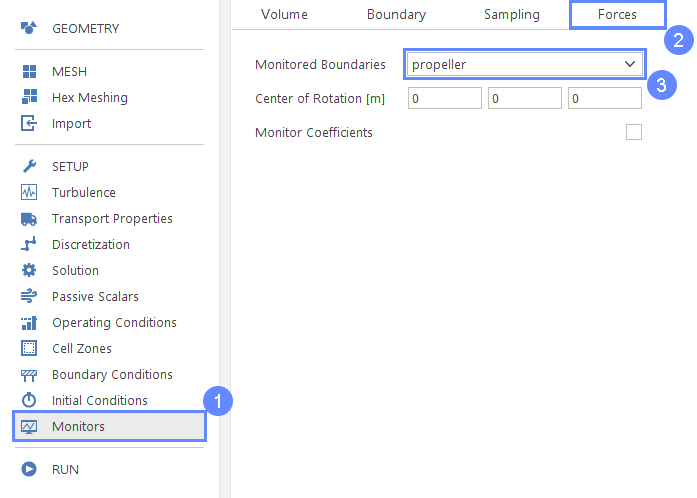
31. Monitor Forces
We will monitor the solution progress by tracking the forces acting on the propeller.
- Go to Monitors panel
- Select Forces tab
- Expand Monitored Boundaries list and select propeller
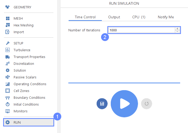
32. Run - Time Control
Finally, we can start our computation.
- Go to Run panel
- Set Number of Iterations to 1000
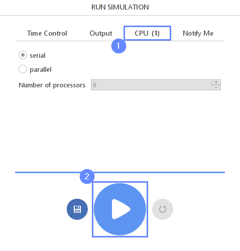
33. Run - CPU
To speed up the calculation process, take advantage of parallel computing and increase the number of CPUs based on your PC’s capability. The free version allows you to use only one processor (serial mode). To get the full version, you can use the contact form to Request 30-day Trial
Estimated computation time for serial mode: 15 minutes
- Switch to CPU tab
- Click Run Simulation button
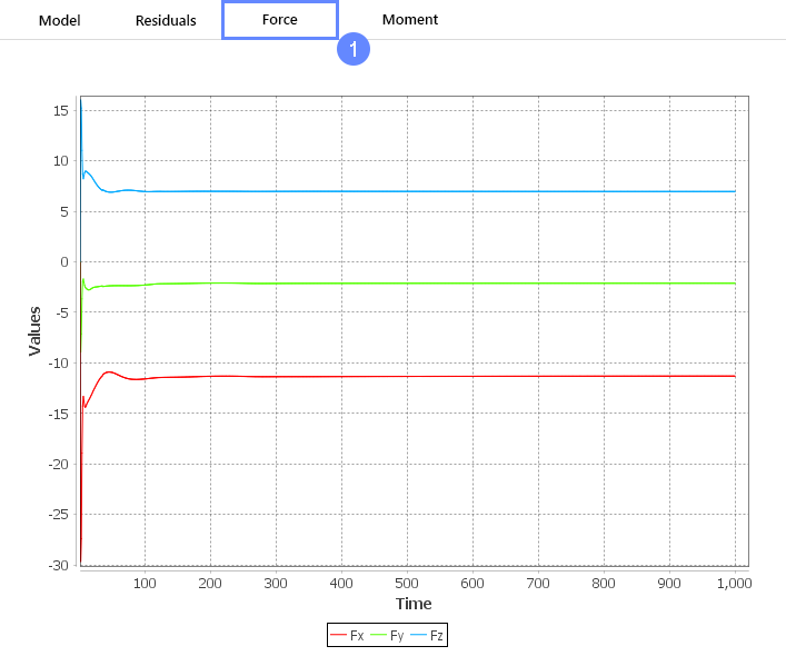
34. Monitor Solution - Force
Check if a solution converges by observing stabilization of forces on the propeller boundary.
- Click on Forces tab to display Force Monitor
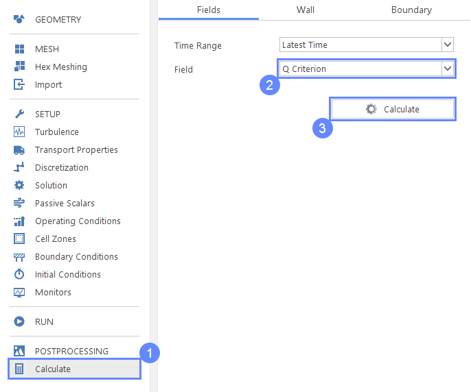
35. Calculate Additional Fields
When a simulation is finished, we want to calculate additional solution field to be used in postprocessing.
- Go to Calculate panel
- Select Q Criterion field
- Calculate the field
Please Note: After clicking the Calculate button, SimFlow will calculate the new flow variable, which will be stored in your project folder and will be accessible in the ParaView.
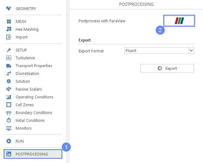
36. Start Postprocessing with ParaView
After computations are finished, we can do complex visualization of our results with ParaView.
- Go to Postprocessing panel
- Run ParaView
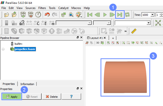
37. ParaView - Load Results
Now we are loading results into the ParaView
- Click Last Frame to select the last result set
- Click Apply to load results into ParaView
- After loading results, they will be shown in the 3D graphic window
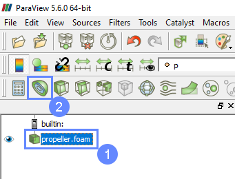
38. ParaView - Display Q Contour (I)
To show the propeller, we will now create a contour.
- Make sure you have your case selected
- Click Contour
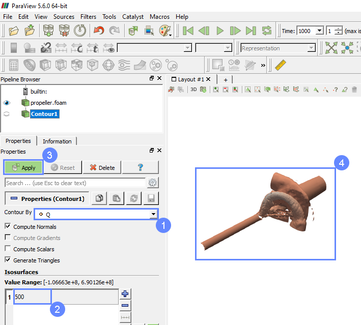
39. ParaView - Display Q Contour (II)
- Set Contour by to Q
- Set contour range to ` 500 ` and click enter
(double click to edit visible value) - Click Apply to create new contour
- After applying changes, the contour will be shown in the 3D window
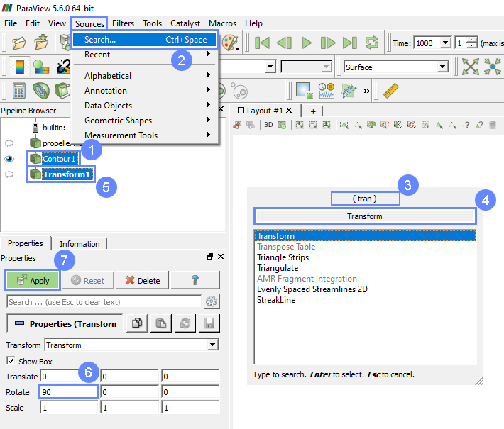
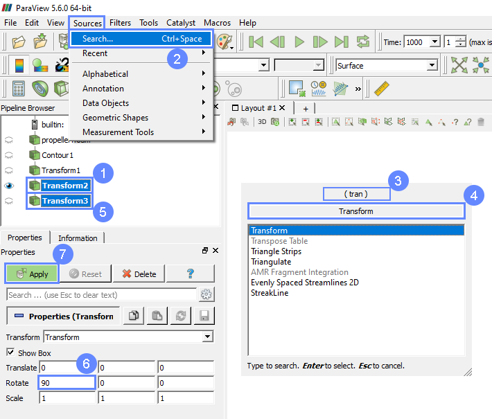
40. ParaView - Show Full Propeller (I)
As you can see, there is only a quarter of the propeller visible and we would like to show the full geometry. In order to do that, we have to duplicate and transform a partial propeller.
- Make sure you have Contour1 selected
- From the Sources Menu select Search option to open a search window
- Start typing the word transform
- Select Transform option
- Make sure you have Transform1 selected
- Define 90 degree rotation about the X axis and click enter
- Click Apply 2 times to create transformation
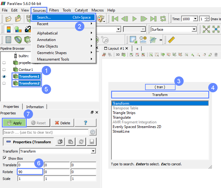
41. ParaView - Show Full Propeller (II)
We have to repeat the previous step to make another transformation - Transorm1 → Transform2
- Make sure you have Transform1 selected
- From the Sources Menu select Search option to open a search window
- Start typing the word transform
- Select Transform option
- Make sure you have Transform2 selected
- Define 90 degree rotation about the X axis and click enter
- Click Apply 2 times to create transformation
42. ParaView - Show Full Propeller (III)
We have to repeat the previous step to make another transformation - Transorm2 → Transform3
- Make sure you have Transform2 selected
- From the Sources Menu select Search option to open a search window
- Start typing the word transform
- Select Transform option
- Make sure you have Transform3 selected
- Define 90 degree rotation about the X axis and click enter
- Click Apply 2 times to create transformation
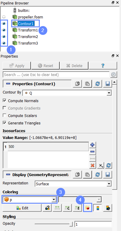
43. Display Full Propeller
To make the full geometry visible, we have to change the visibility of all geometries
- Make sure the contour and all its transformations are visible
- Select Contour1
- Choose pressure p from the coloring list
- Click Toggle Color Legend Visibility and choose Blue to Red Rainbow
- Choose pressure p for the remaining quarters
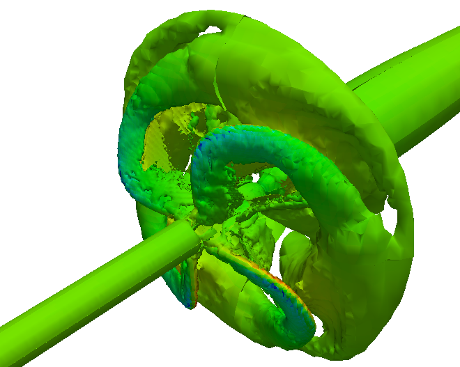
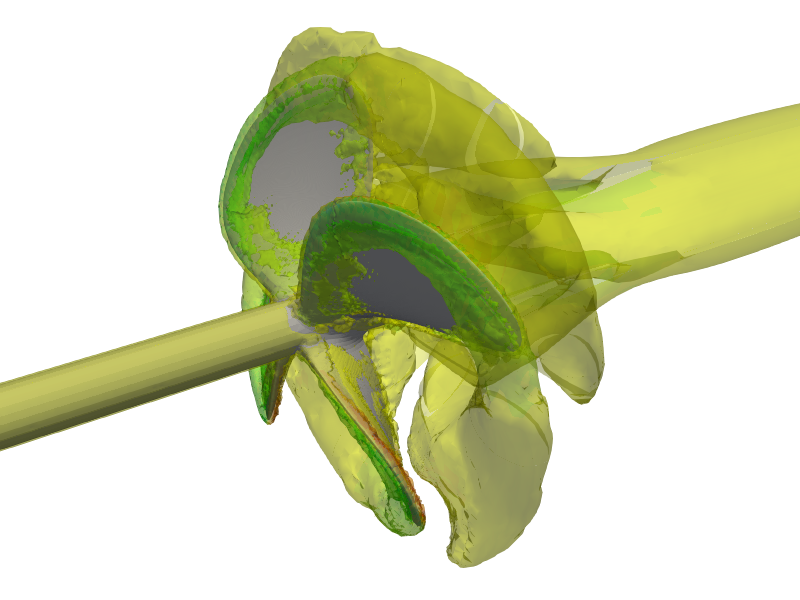
44. Final Results
In the 3D view, the contour of full propeller should appear