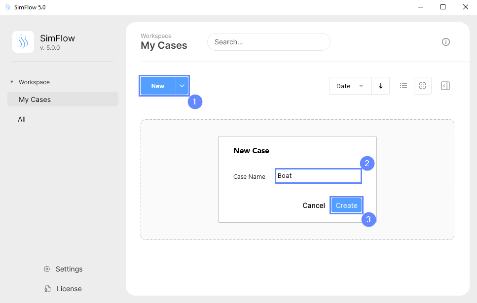
3. Create Case
Open SimFlow and create a new case named Boat
- Click New
- Provide name Boat
- Click Create to open a new case
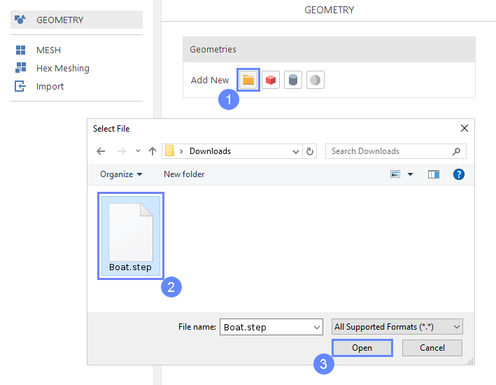
4. Import Geometry - Boat
Firstly we need to Download GeometryBoat. The geometry will be imported in the same units as it was exported to the STEP format.
- Click Import Geometry
- Select geometry file
Boat.step - Click Open
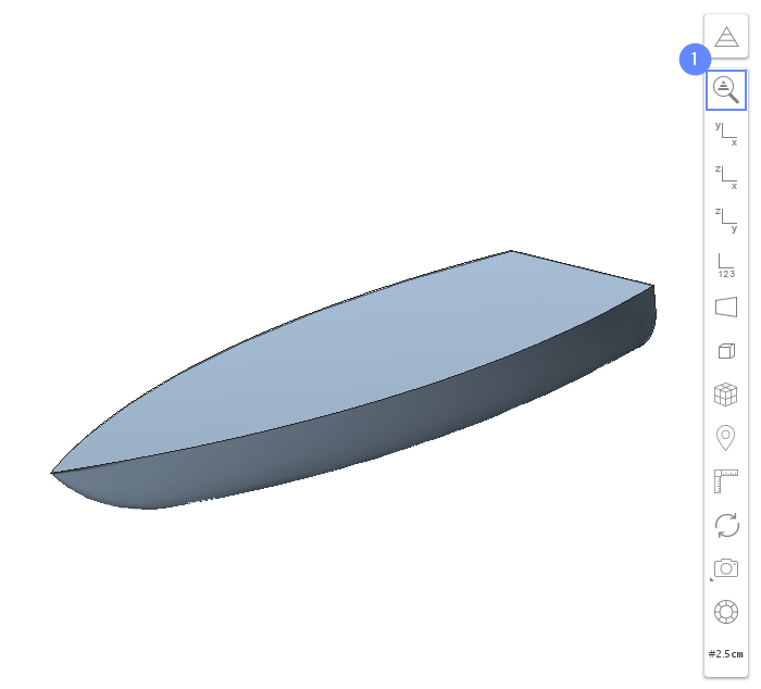
5. Preview Geometry - Boat
After importing geometry, it will appear in the 3D window.
- Click Fit View to zoom in on the geometry.
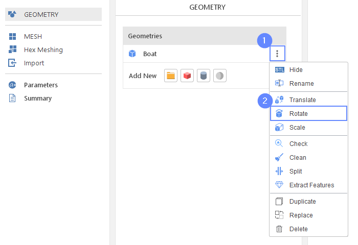
6. Rotate Geometry - Boat (I)
We will rotate the model about X axis at 90 deg to orient the Z axis vertically.
- Expand the Options list for
Boat - Select Rotate
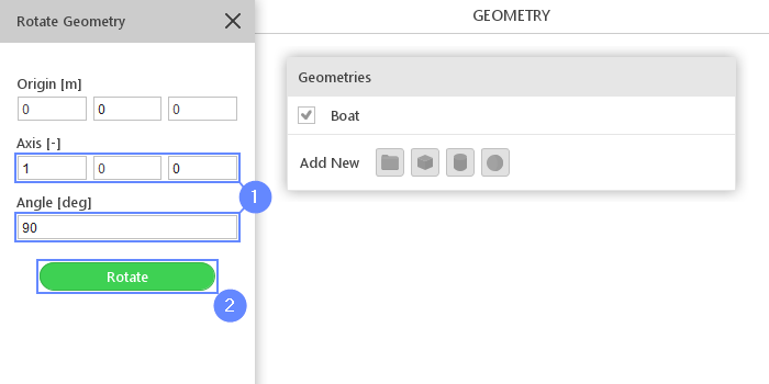
7. Rotate Geometry - Boat (II)
- Set the following parameters accordingly
Axis \({\sf [-]}\)100
Angle \({\sf [deg]}\)90 - Click Rotate
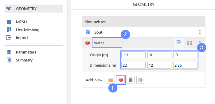
8. Create Geometry - Water
Additionally, to the hull geometry, we will create a box that will be used to indicate the initial water location.
- Select Create Box
- Change geometry name from
box_1to water
double click to edit name and press Enter to confirm - Set the origin and box dimensions:
Origin \({\sf [m]}\)-11-6-3
Dimensions \({\sf [m]}\)22122.85
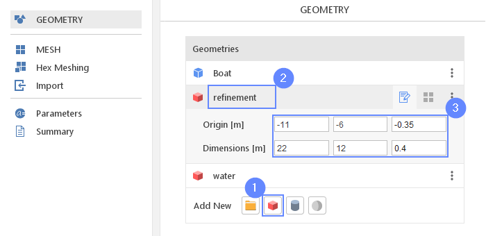
9. Create Geometry - Refinement
We need to refine the mesh near the water surface to increase the accuracy of the results. For this purpose, we will create also a refinement box.
- Select Create Box
- Change geometry name from
box_1to refinement - Set the origin and box dimensions
Origin \({\sf [m]}\)-11-6-0.35
Dimensions \({\sf [m]}\)22120.4
10. Meshing Parameters - Boat
In order to create the mesh, we need to specify geometries options for the meshing process.
- Go to
Hex Meshingpanel - Select
Boatgeometry - Enable Mesh Geometry
- Enable Create Boundary Layer Mesh
- Set
RefinementtoMin 4Max 4 - Set
No. of Layersto 4
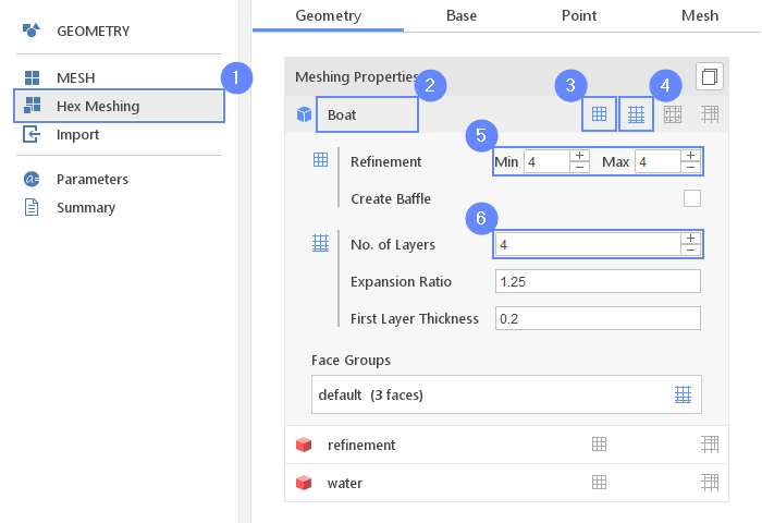
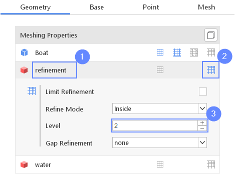
11. Meshing Parameters - Refinement
- Click on the
refinementgeometry - Enable Refine Geometry
- Set the refinement
Levelto 2
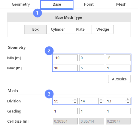
12. Base Mesh - Domain
Now, we will define the base mesh. The box geometry determines the background mesh domain. The model is symmetrical with respect to the XZ plane and we can take advantage of this fact. Using box dimensions we will choose only half of the required domain.
- Go to
Basetab - Set the size of the base mesh:
Min \({\sf [m]}\)-100-2
Max \({\sf [m]}\)1051 - Define the number of divisions
Division551413
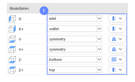
13. Base Mesh - Boundaries
We need to assign individual names to each side of the base mesh. This will allow us to apply different conditions to each side.
- Define boundary names and types accordingly
X-inletpatch
X+outletpatch
Y-symmetrysymmetry
Y+symmetrysymmetry
Z-bottomwall
Z+toppatch
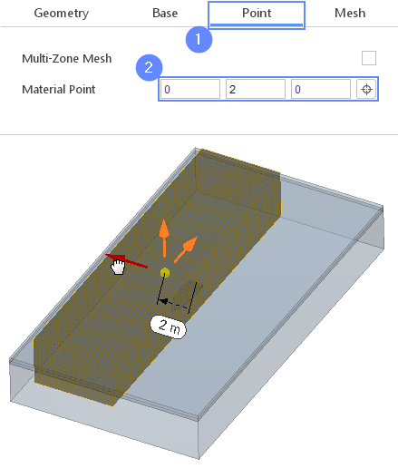
14. Material Point
Material Point tells the meshing algorithm on which side of the geometry the mesh is to be retained. Since we are considering fluid outside the boat, we need to place the material point outside the geometry.
- Go to
Pointtab - Specify location inside base mesh, but outside boat geometry
Material Point020
| You can specify the point location from the 3D view. Hold the Ctrl key and drag the arrows to the destination. |
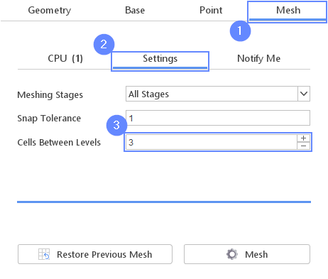
15. Meshing Settings
We can define the count of the buffer cells between refinement levels.
This parameter determines the width of the transition zone between refined and background mesh. Lowering this parameter will reduce the overall cells count.
- Go to
Meshtab - Go to
Settings - Set
Cells Between Levelsto 3
16. Start Meshing
In this step we will initiate the meshing process.
In the meshing panel you may indicate how many CPUs would you like to use for this process. Please note that if you are using SimFlow free version you may only use serial meshing, and you may not create meshes larger than 200'000 nodes.
If you would like to test full version Request 30-day Trial
- Go to
CPUtab - Press the Mesh button to start meshing process

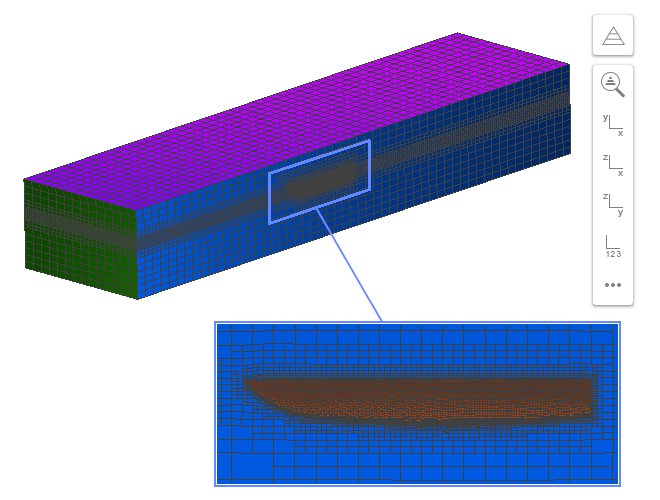
17. Mesh
After the meshing process is finished, the mesh will appear in the graphics window.
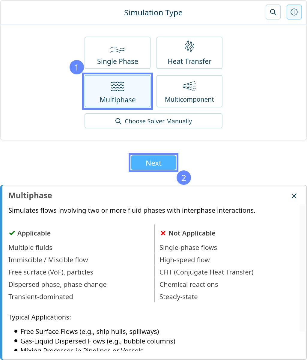
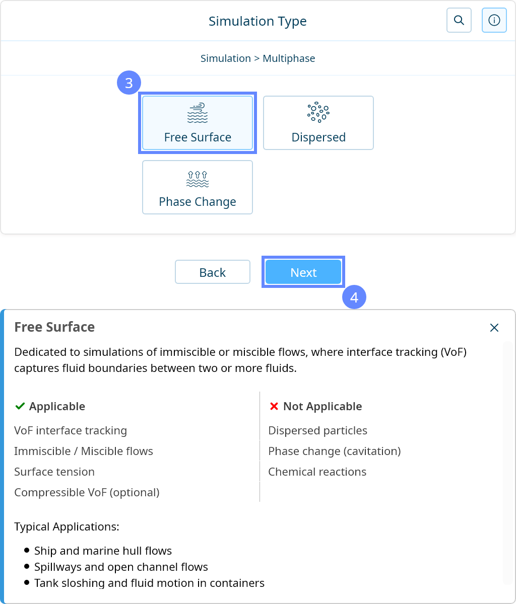
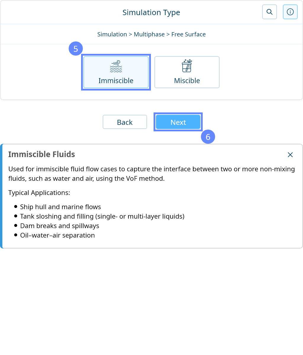
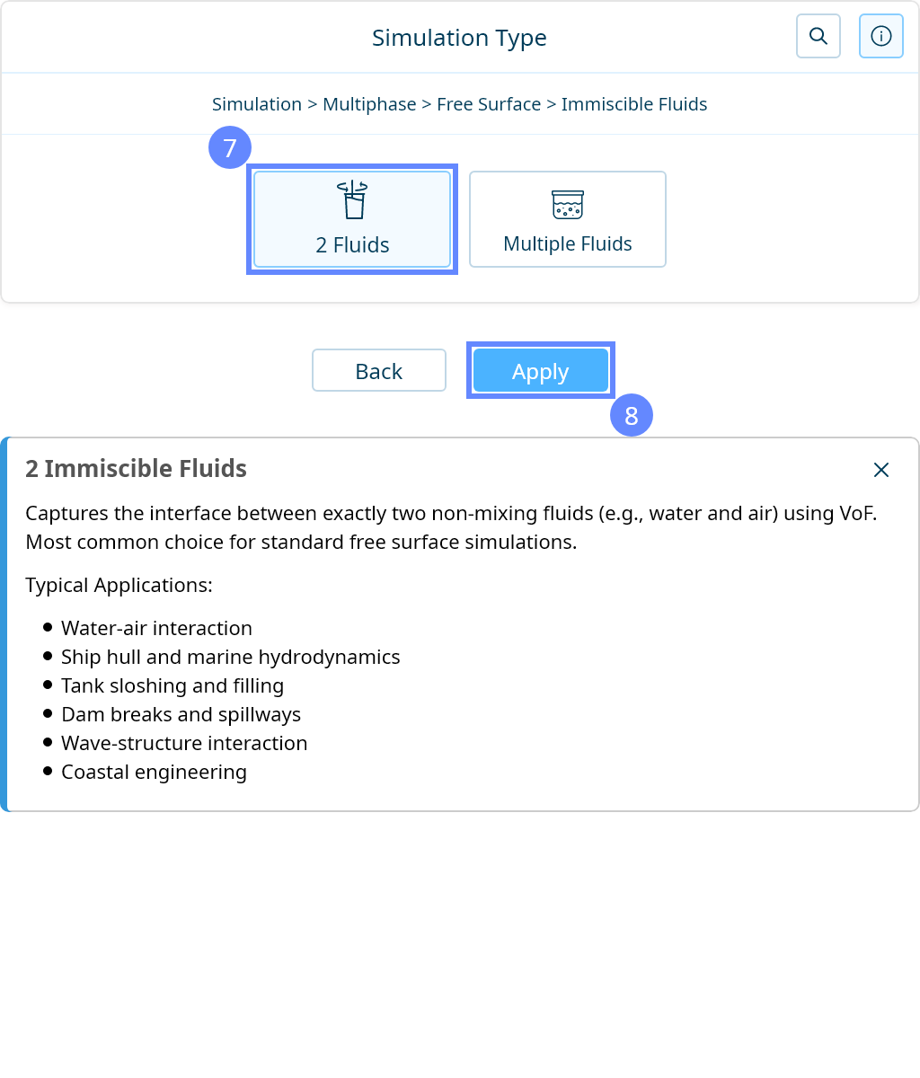
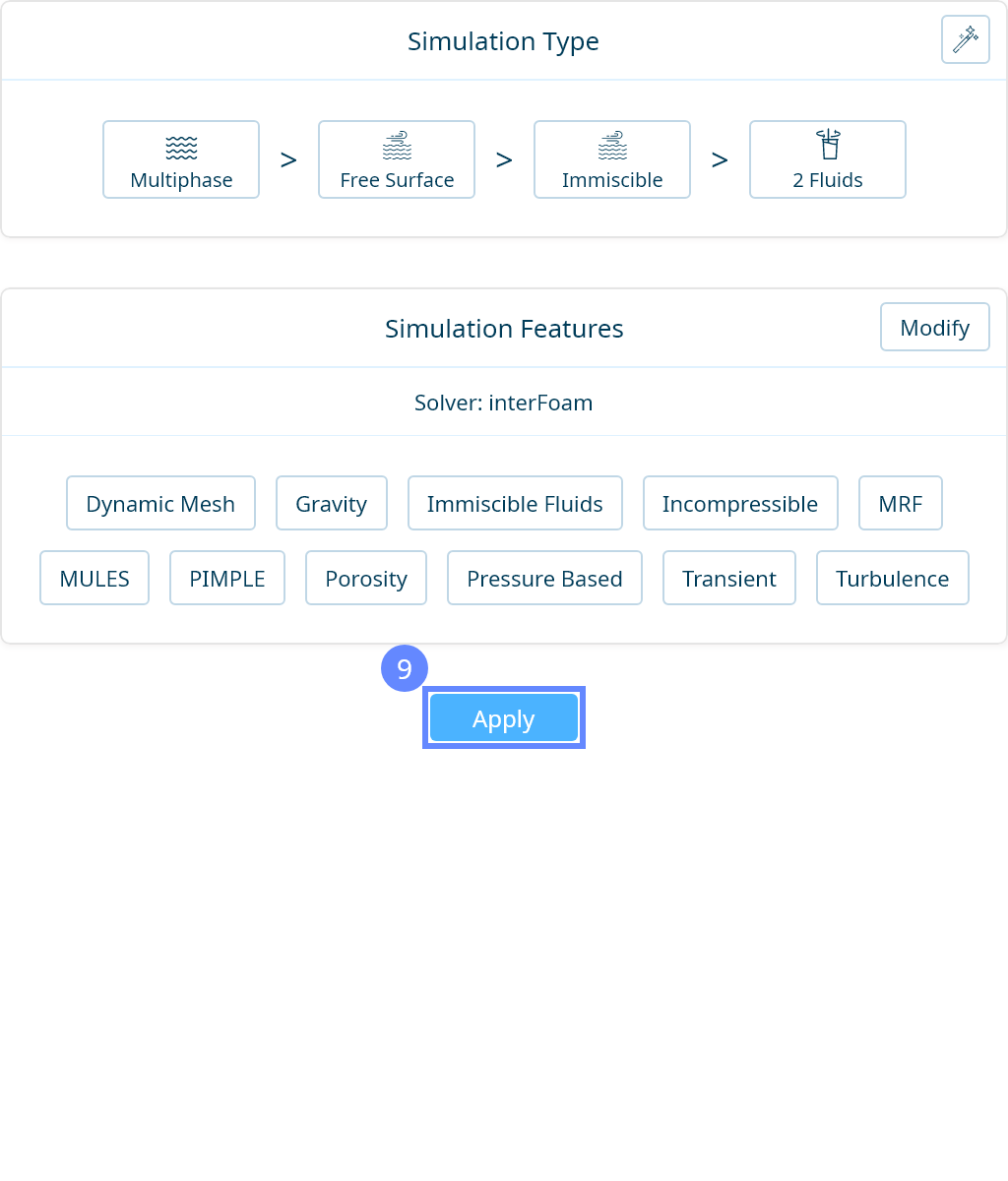
18. Simulation Type
We want to analyze the flow around a ship hull with a free surface. For this purpose, we will use a transient simulation of two immiscible fluids (water and air) using the free-surface method.

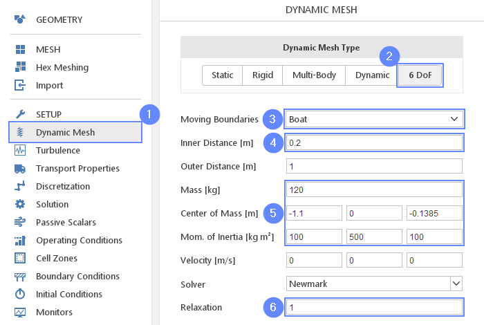
19. Dynamic Mesh (I)
The dynamic mesh can be used for a simulation where the shape of the domain is changing. In our case, we will use dynamic mesh capabilities paired with six degrees of freedom (6 DOF) solver.
The 6DOF solver will predict the trajectory of a moving body using the aero or hydrodynamic forces and inertial properties assigned to a given boundary. During the analysis, the mesh will adjust to the new position of the body by moving nodes in the deformation region defined by the distance from the body.
- Go to
Dynamic Meshpanel - Choose
Dynamic Mesh Type6 DoF - Select the
Boatgeometry - Set the
Inner Distance [m]to 0.2 for the deformation region - Set the boat mass properties
Mass \({\sf [kg]}\)120
Center of Mass \({\sf [m]}\)-1.10-0.1385
Mom. Of Inertia \({\sf [kg m^2]}\)100500100 - Set the
Relaxationto 1
| We use only half of the mass because of model symmetry |
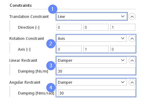
20. Dynamic Mesh (II)
It is possible to constrain boundary motion. We will allow the boat to move only in the Z-axis direction and rotate about Y-axis. We will also enable damping to improve the stability of the calculation.
- 2 Set the constraints accordingly
Translation ConstraintLine
Rotation ConstraintAxis
Axis \({\sf [-]}\)010 - 3 Set the restraints accordingly
Linear RestraintDamper
Damping \({\sf [Ns/m]}\)30
Angular RestraintDamper
Damping \({\sf [Nms/m]}\)30
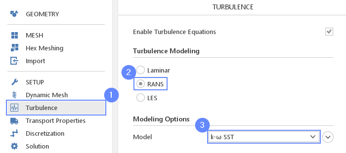
21. Turbulence
For the purpose of this tutorial, we will model the turbulence phenomenon using the k-ω SST model.
- Go to
Turbulencepanel - Select
RANSturbulence formulation - Select \(k {-} \omega \; SST\) model
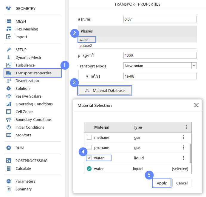
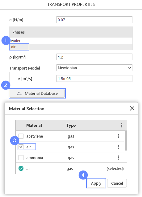
22. Transport Properties - Water
In order to define water and air, we need to go to the transport properties panel, and use predefined fluids properties from the material database.
- Go to
Transport Propertiespanel - Change phase name from
phase1to water - Open Material Database
- Pick up
waterfrom the list - Click Apply
23. Transport Properties - Air
Repeat previous step for phase2 using air properties.
To assign material to the domain, the phase fraction parameter \(\alpha_{phase}\) is used. The parameter determines the proportion of each fluid in the domain.
The value of phase fraction varies in range from 0 to 1 where \(\alpha_{phase 1}=1\) means that the whole domain is filled only with the phase1, while \(\alpha_{phase 1}=0\) means that the domain is filled with the second phase.
We will assign \(\alpha_{phase}\) parameter in the later steps.
- Change phase name from
phase2to air - Open Material Database
- Pick up
airfrom the list - Click Apply
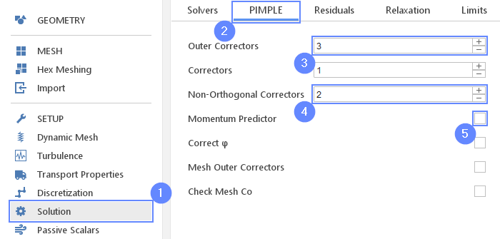
24. Solution - PIMPLE
For the purpose of the simulation we will change PIMPLE algorithm parameters to increase stability:
- Go to
Solutionpanel - Switch to the
PIMPLEtab - Increase
Outer Correctorsto 3 - Increase
Non-Orthogonal Correctorsto 2 - Uncheck
Momentum Predictorfor stability
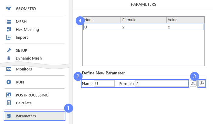
25. Simulation Parameters
The velocity magnitude will be used in multiple simulation settings. It is handy to parameterize velocity value to be easily accessible in the future.
- Go to
Parameterspanel - Define new parameter
NameU
Formula2 - Press Enter or Create Parameter button
- The newly created parameter will be shown in the parameters list
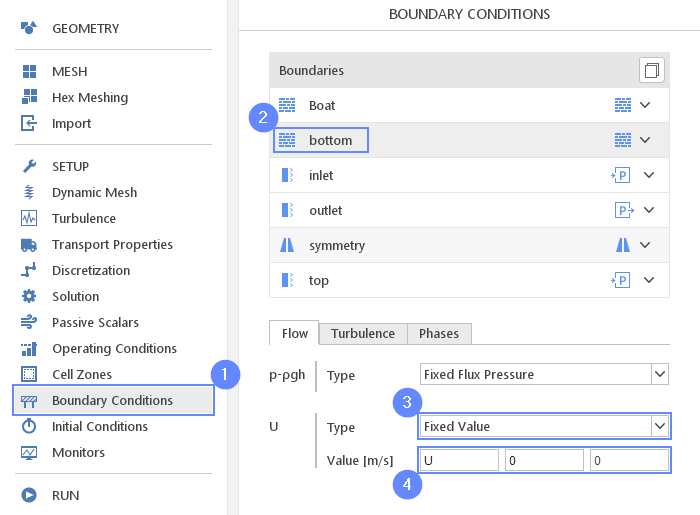
26. Boundary Conditions - Bottom
In our simulation, the frame of reference will be associated with the boat and therefore we will simulate a fluid flow around the stationary boat. In order to properly represent ground in the boat frame of reference, we will enforce velocity at the bottom mesh boundary.
- Go to
Boundary Conditionspanel - Select the
bottomboundary - Change the
Typeof velocity to theFixed Value - Set the Value \({\sf [m/s]}\)U00
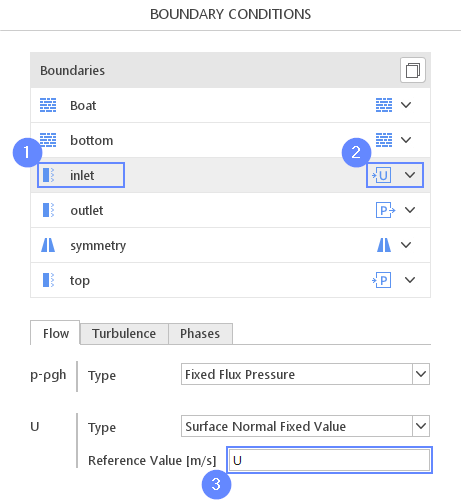
27. Boundary Conditions - Inlet (Flow)
To model the inlet to the domain, we will assign the Inlet Velocity character and use the value of the "U" parameter as the inlet velocity value.
- Select the
inletboundary - Set the Velocity Inlet character
- Set the velocity
Reference Value [m/s]to U
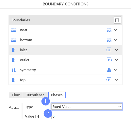
28. Boundary Conditions - Inlet (Phases)
In addition to setting the flow conditions, selecting the inlet phase is also necessary.
Initially, we will specify pure air as the inlet phase. The water phase at the inlet will be patched later on by the water box geometry. Patching operation will modify the value parameter in a certain region, and effectively we will get an inlet of two phases from a single boundary.
- Switch tab to
Phases - Set the type to
Fixed Value
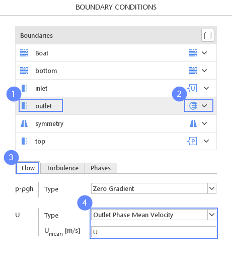
29. Boundary Conditions - Outlet (Flow)
For the outflow boundary we will use Outlet Phase Mean Velocity condition. This boundary condition adjusts the velocity for the given phase to achieve the specified mean velocity.
- Select the
ouletboundary - Set the
Outflowcharacter - Switch tab to
Flow - Set the velocity type and mean value accordingly
UTypeOutlet Phase Mean Velocity
UUmean \({\sf [m/s]}\)U
| After you change flow boundary condition, the character will switch form Outflow to Custom. Do not change it back to Outflow afterwards. |
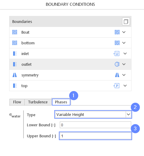
30. Boundary Conditions - Outlet (Phases)
- Switch tab to
Phases - 3 Set the \(\alpha_{water}\) parameters accordingly
\(\alpha_{water}\)TypeVariable Height
\(\alpha_{water}\) Upper Bound \({\sf [-]}\)1
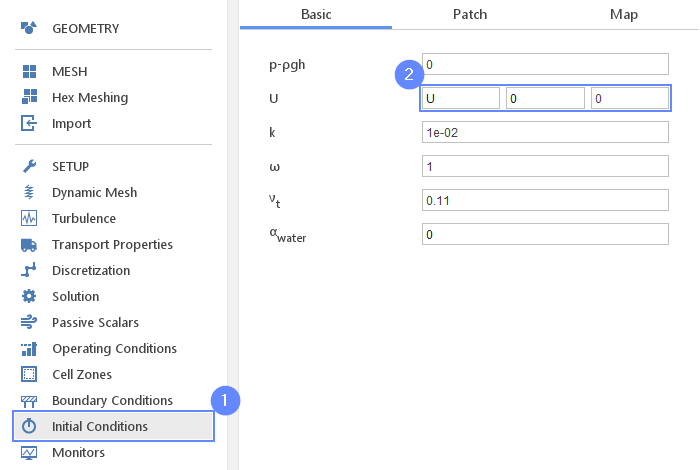
31. Initial Conditions - Basic
Before we start simulation, we need to define the initial state.
We will use parameter U to initiate constant velocity in the domain. The domain will initially be filled entirely with air, as indicated by a phase fraction \(\alpha_{air}=0\).
- Go to
Initial Conditionspanel - Set the velocity to U00
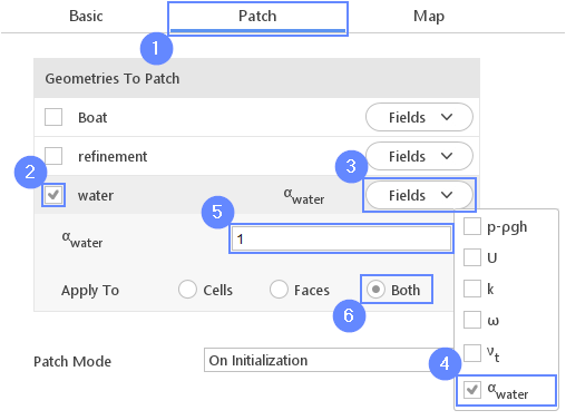
32. Initial Conditions - Patch
Using the water geometry, we will overwrite the phase fraction value inside it. We will set the \(\alpha_{water}\) to 1 to fill the patched geometry with the water.
- Switch to
Patchtab - Enable initialization on
watergeometry - Expand Fields list
- Select \(\alpha_{water}\) fraction for initialization
- Set initial value of \(\alpha_{water}\) to 1
- Apply patch for
Bothcells and faces. This will override values at boundaries as well.
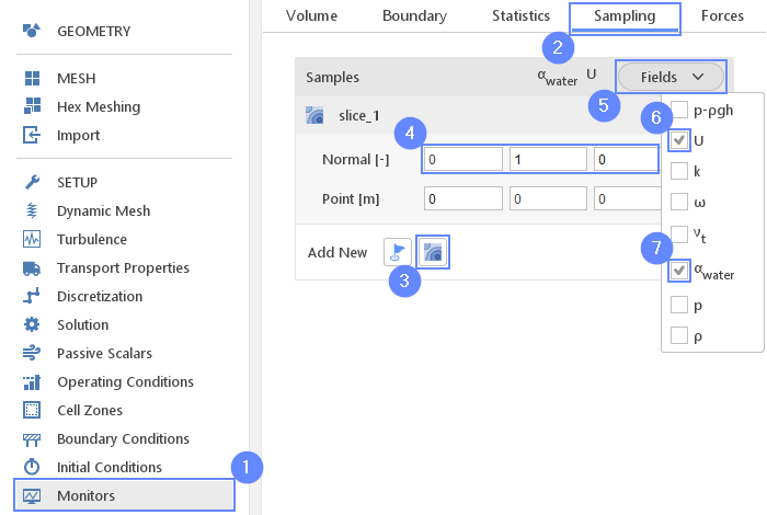
33. Monitors - Sampling
During calculation, we can observe intermediate results on a section plane.
To add sampling data on a plane we need to define plane properties and also select fields that will be sampled. Note that runtime post-processing can only be defined before starting calculations and can not be changed after the simulation has started.
- Go to
Monitorspanel - Switch to
Samplingtab - Select Create Slice
- Set the slice normal vector align y-axis
Normal \({\sf [-]}\)010 - Expand Fields list
- Check the velocity
U - Check the water phase \(\alpha_{water}\)
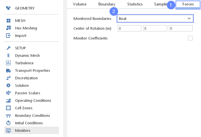
34. Monitors - Forces
Additionally, we will observe forces acting on the boat boundary.
- Switch to
Forcestab - Expand
Monitored Boundarieslist and checkBoat
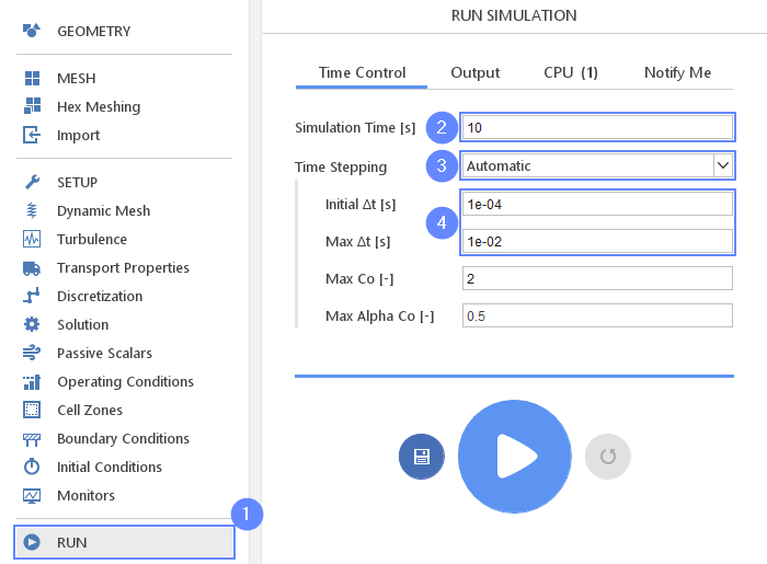
35. Run - Time Control
For any simulation, it is very convenient to let the solver automatically determine the proper time step value. To use this option, we need to define time step constraints by providing the initial time step(adjusted by the solver during computations) and maximal time step value. The rest of the parameters we can leave the default.
- Go to
RUNpanel - Set the
Simulation Time [s]to 10 - Change
Time SteppingtoAutomatic - Set initial and maximum timesteps (solver will start computation with the initial value and adjust it in the next iterations not exceeding the maximum value)
Initial \(\Delta t\) \({\sf [s]}\)1e-04
Max \(\Delta t\) \({\sf [s]}\)1e-02
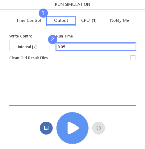
36. Run - Output
We can control how often results should be saved on the hard drive. Only this data will be available for postprocessing.
- Switch to
Outputtab - Set the
Write ControlInterval [s]to 0.05
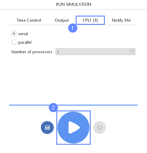
37. Run - CPU
To speed up the calculation process, take advantage of parallel computing and increase the number of CPUs based on your PC’s capability. The free version allows you to use only one processor (serial mode). To get the full version, you can use the contact form to Request 30-day Trial
Estimated computation time for serial mode: over 5 hours
- Switch to CPU tab
- Click Run Simulation button
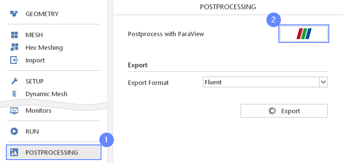
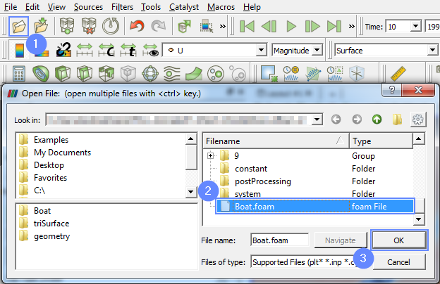
38. Postprocessing - ParaView
Once the computations have been completed, we can perform advanced visualization of the results using ParaView.
- Go to
POSTPROCESSINGpanel - Click on Run ParaView
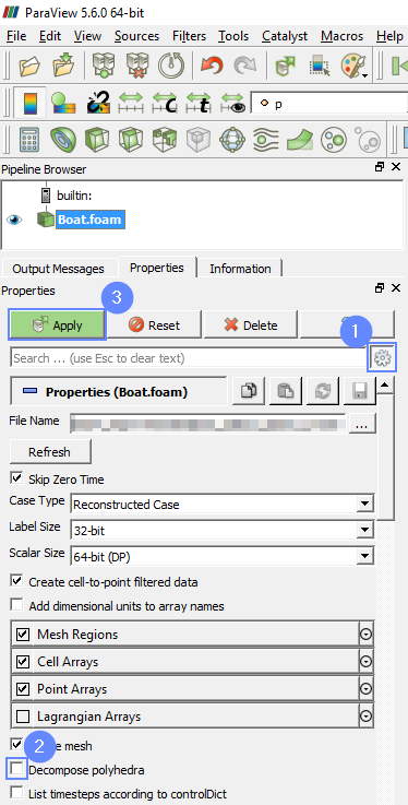
39. ParaView - Load Results
Load the results into the program.
- Turn on Toggle advanced properties
- Uncheck option
Decompose polyhedra - Click Apply to load results into ParaView
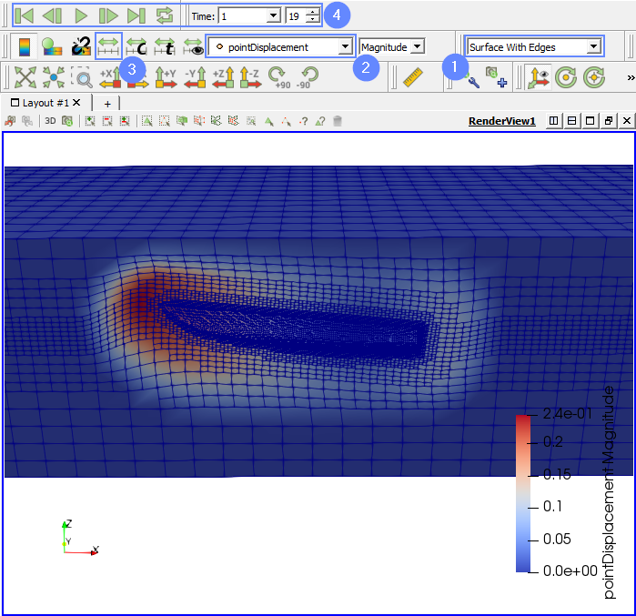
40. ParaView - Dynamic mesh
We will look at the dynamic mesh displacement.
As we can see, the boat can move along Z-axis and rotate around Y-axis. The mesh at a distance of 0.2 m from the boat is rigid and moves together with a boat. The mesh at the distance from 0.2 m to 1 m from the boat is able to move. Further than 1 m from the boat, the mesh is non-deformable.
- Select
Surface with Edgesfrom the representation toolbar list - Select
pointDisplacementfrom the variable list - Click Rescale to Data Range
- Play with an animation buttons to track the results of analysis
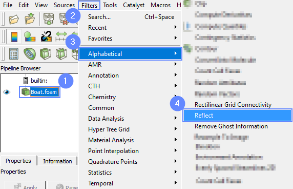
41. ParaView - Reflect the results (I)
During the simulation, only one half of the fluid domain was used. However, during the post-processing stage, we can replicate the second half of the domain.
To produce a visualization that is symmetrical, we will reflect the results across the plane of symmetry.
- Select the case
Boat.foam - Extend the list of
Filtersfrom the top menu - Go to
Alphabetical - Select
Reflectfrom the list
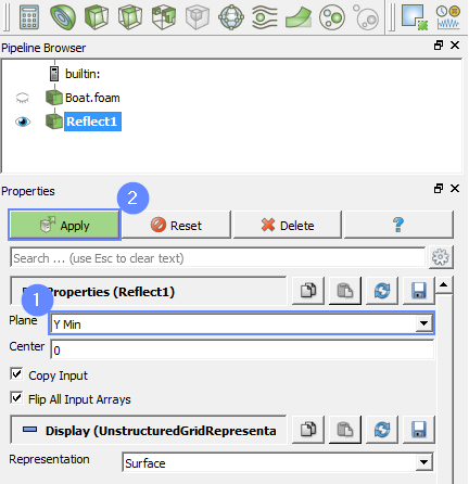
42. ParaView - Reflect the results (II)
- Choose the plane of the reflection
Y min - Click Apply
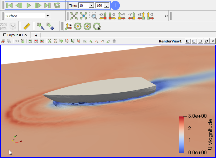
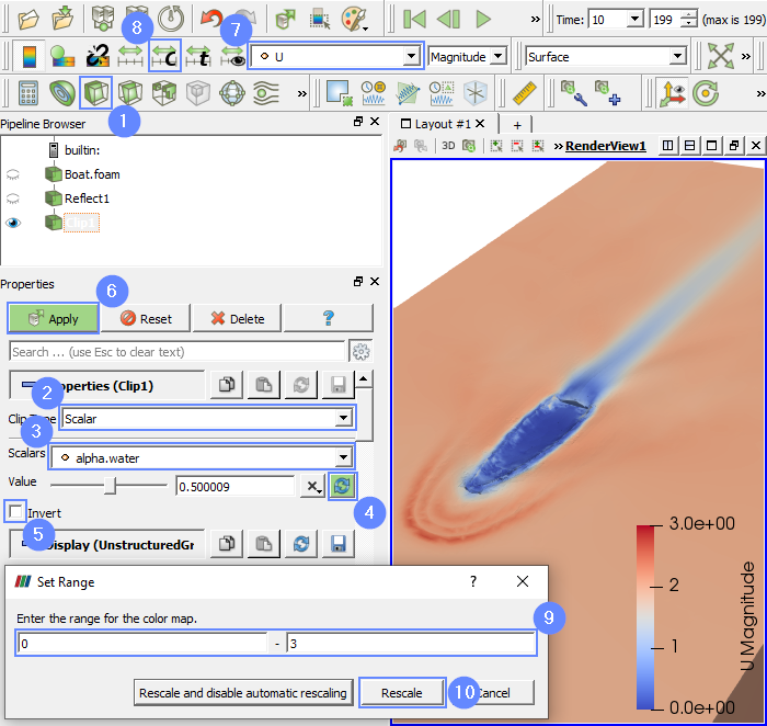
43. ParaView - Water Surface
We will focus on the water-air interface behaviour and observe the velocity map.
- Select Clip from top menu
- Change the clip type to
Scalar - Select
alpha.waterfrom the scalar list - Click Refresh
- Make sure
Invertoption is unchecked - Click Apply
- Select the velocity
Ufrom the list - Click on Rescale to Custom Data Range
- Set the range from 0 to 3
- Confirm by clicking Rescale
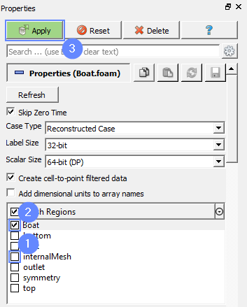
44. ParaView - Boat Geometry (I)
To display the boat geometry, we will read the result file once again and load only the boat boundary.
- Select Open from top menu
- Choose the
Boat.foamfile from case folder - Press OK
45. ParaView - Boat Geometry (II)
- Uncheck
internalMeshfrom theMesh Regions - Check the
Boat - Press Apply
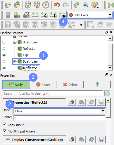
46. ParaView - Boat Geometry (III)
Similarly as before, we will reflect the boat geometry.
- Select the new case name
Boat.foam, go toFilters, extendAlphabeticaland selectReflectfrom the list - Choose the plane of reflection
Y min - Click Apply
- Select the
Solid Colorfrom the list
47. ParaView - Results
- Play with animation buttons to investigate the time history of the flow.