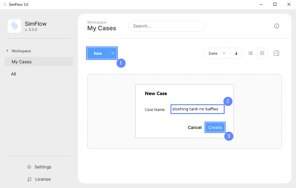
3. Create Case
Open SimFlow and create a new case named sloshing tank no baffles
- Click New
- Provide name sloshing tank no baffles
- Click Create to open a new case
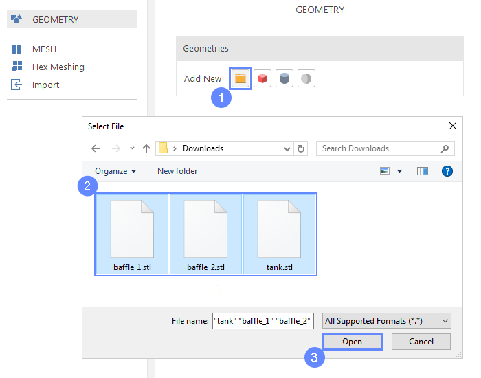
4. Import Geometry - Tank
Although the baffles are not involved in the first simulation we will import them at this stage. We can omit them when creating the first mesh and include them in the second simulation.
- Click Import Geometry
- Select geometry files: baffle_1.stl baffle_2.stl tank.stl
- Click Open
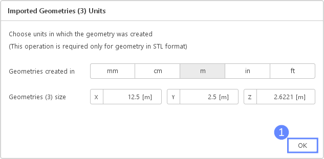
5. Imported Geometry Units
The STL format does not contain the unit information which are defined during the geometry export. Therefore, you must manually specify the correct unit after import. If we do not know the exported unit, we can estimate it based on the total size of the model. The size is displayed next to Geometry size label. In our case, the default unit meter is correct.
- To confirm default unit meter, press OK
6. Display Geometry
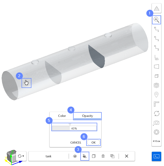
Inside the tank, there are two baffles. To view the baffles, we will reduce tank opacity.
- Click Fit View and orient the model using mouse buttons
- Hold the Ctrl key and select the tank geometry by clicking on it with the left mouse button. Selected geometry will be highlighted in red
- Click Change Object Display Properties button
- Switch the tab to Opacity
- Set the opacity to
40% - Approve by clicking OK
- Press Esc or click the X button to exit selection mode
7. Split Geometry - Tank (I)
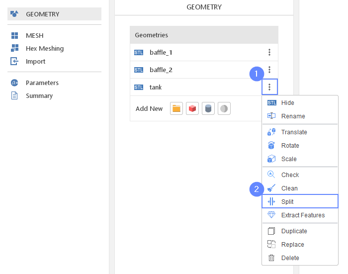
The imported geometry is made up of a single surface. We need to split it into multiple faces for further processing.
- Extend Options list next to the tank geometry
- Select Split
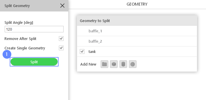
8. Split Geometry - Tank (II)
- Select Split
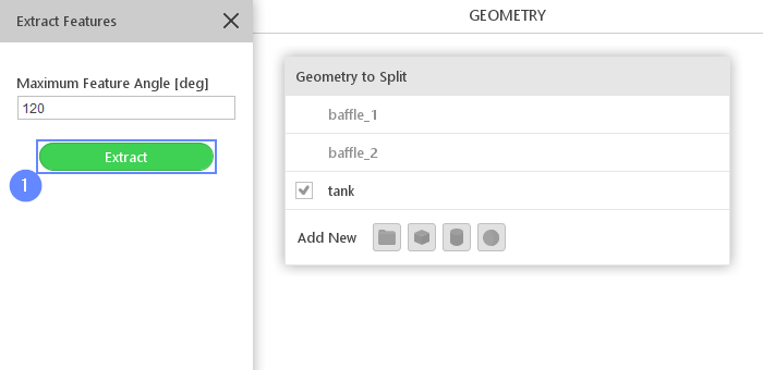
9. Extract Geometry - Tank (I)
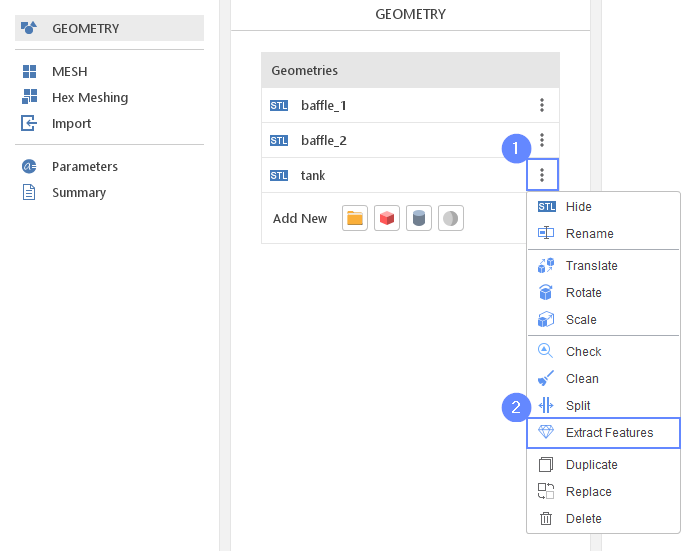
To make sharp edges visible, we will use Extract Features operation. These edges will indicate additional mesh refinement regions.
- Extend Options list next to the tank geometry
- Select Extract Features
10. Extract Geometry - Tank (II)
- Select Extract
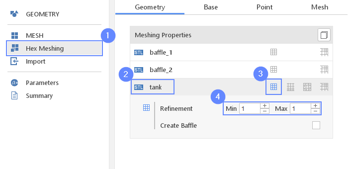
11. Meshing Parameters - Tank
In order to create the mesh, we need to specify geometries options used during the meshing. In this tutorial, we will analyze two configurations: with and without baffles. We will start with the tank itself and skip baffles for now.
- Go to Hex Meshing panel
- Select tank
- Enable Mesh Geometry
- Set Refinement to Min 1 Max 1
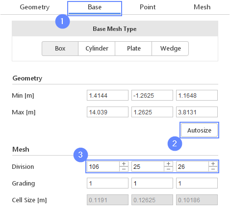
12. Base Mesh
Now we will define the base mesh. The box geometry determines the background mesh.
- Go to Base tab
- Click on Autosize
- Define the number of divisions
Division1062526
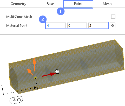
13. Material Point
Material Point indicates the meshing algorithm on which side of the geometry the mesh is to be retained. Since we are considering fluid inside the tank we need to place the material point inside the geometry.
- Go to Point tab
- Specify location inside tank geometry
Material Point402
You can specify the point location from the 3D view. Hold the CTRL key and drag the arrows to the destination.
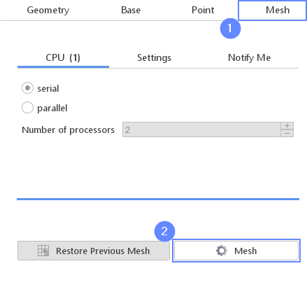
14. Start Meshing
Everything is now configured and ready to be meshed.
- Go to Mesh tab
- Press the Mesh button to start meshing process
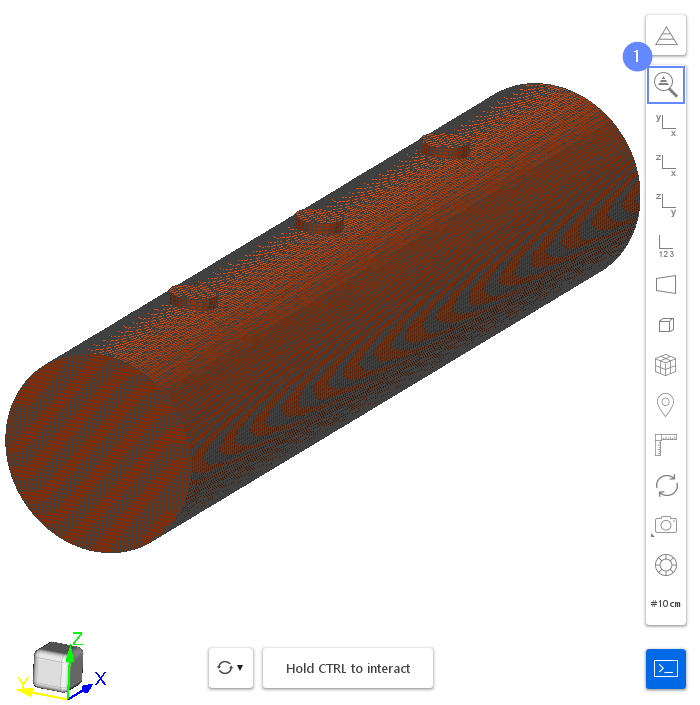
15. Examine Mesh
After the meshing is finished the mesh will appear in the graphics window. The mesh should consist of only a single boundary.
- Click Fit View
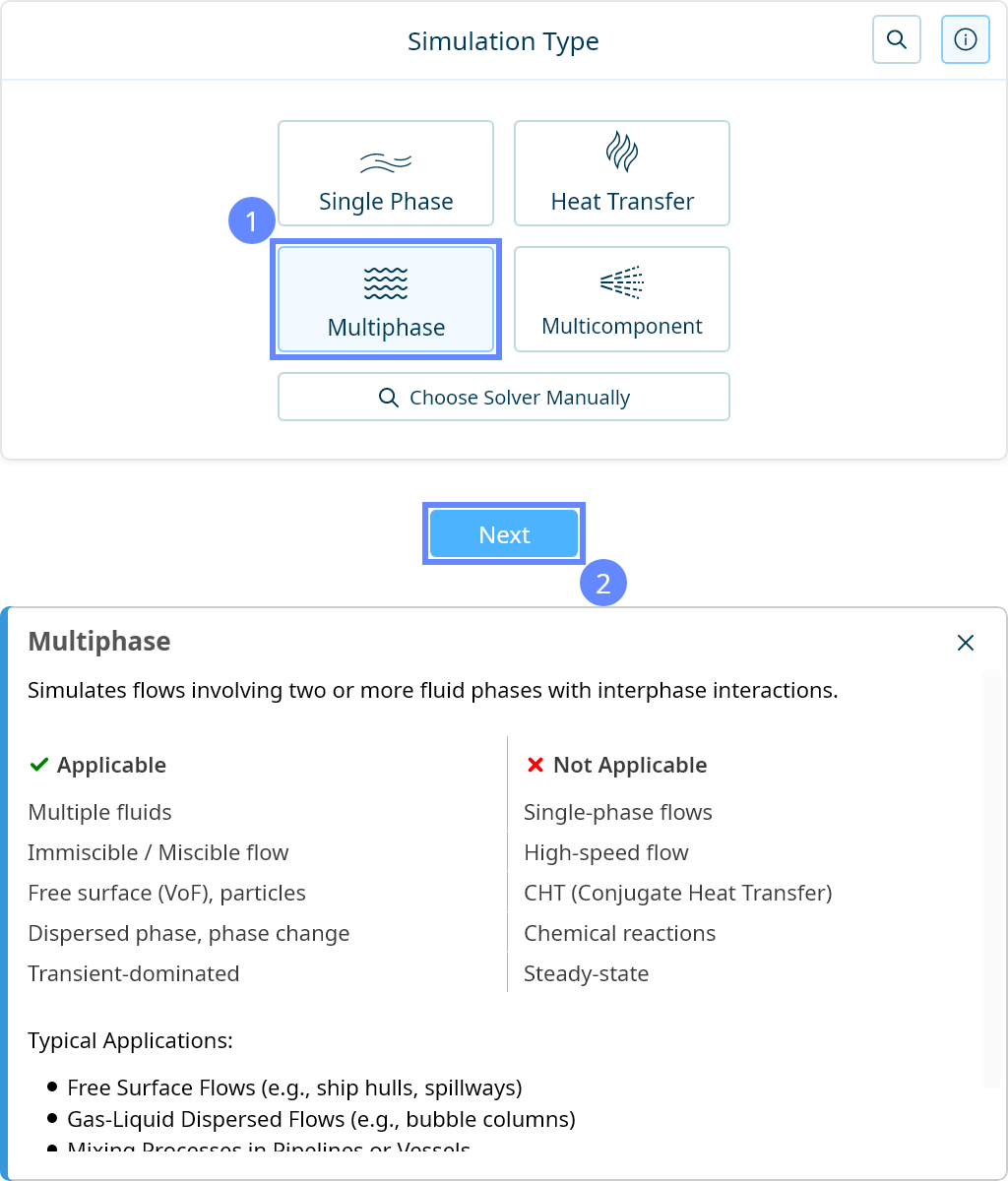
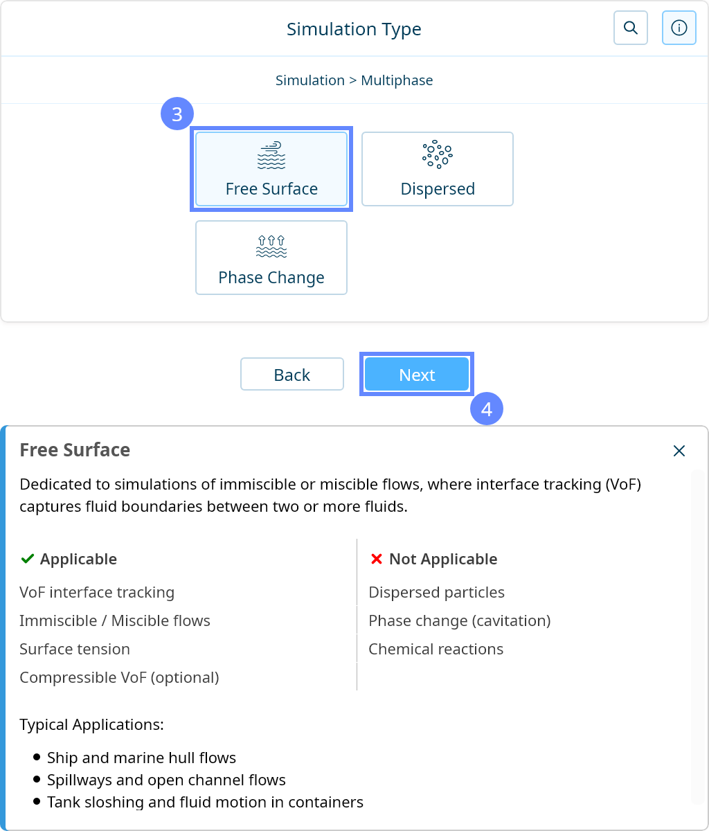
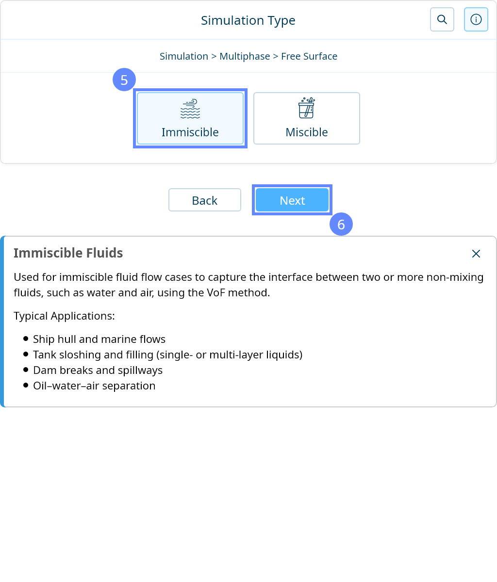
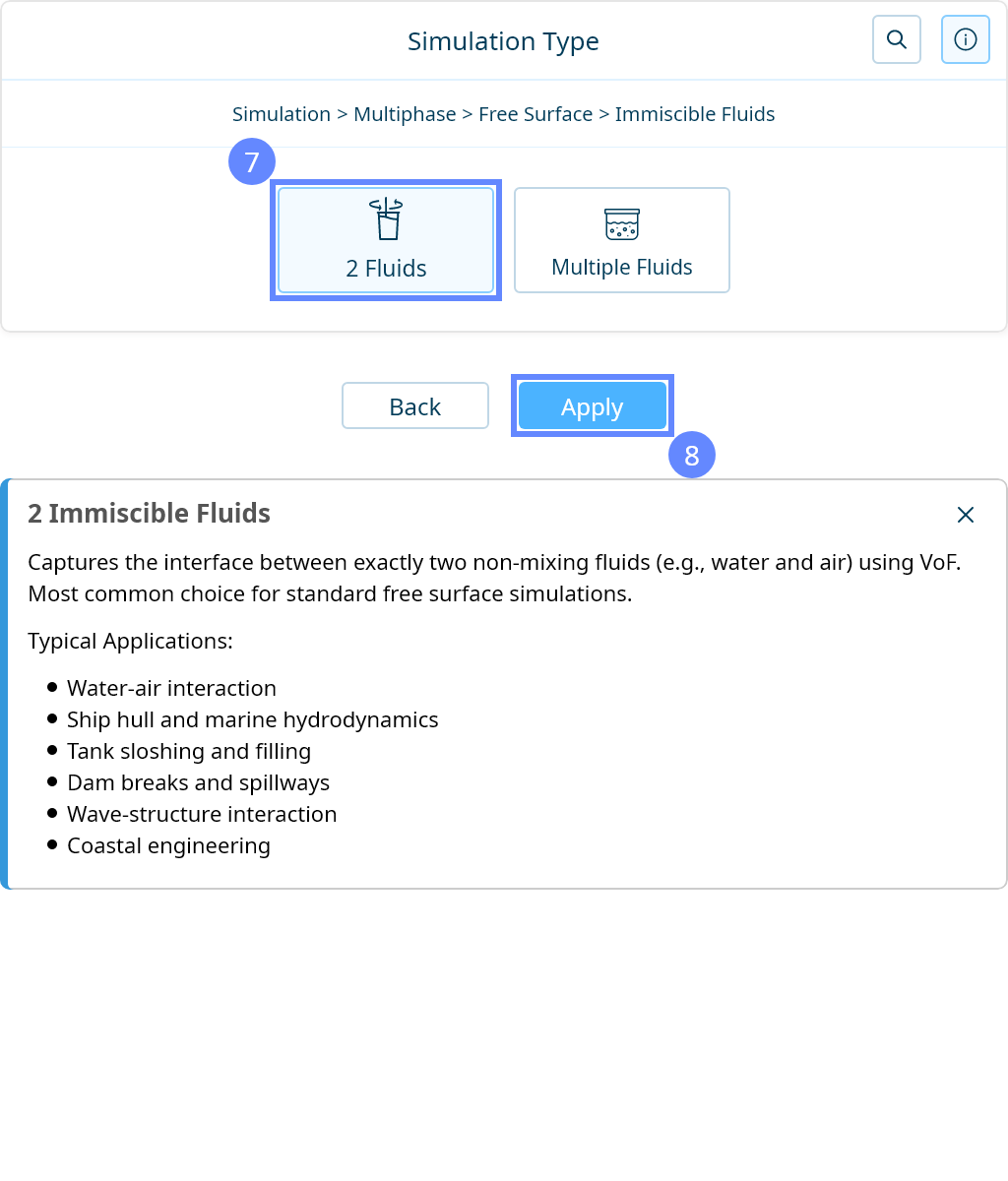
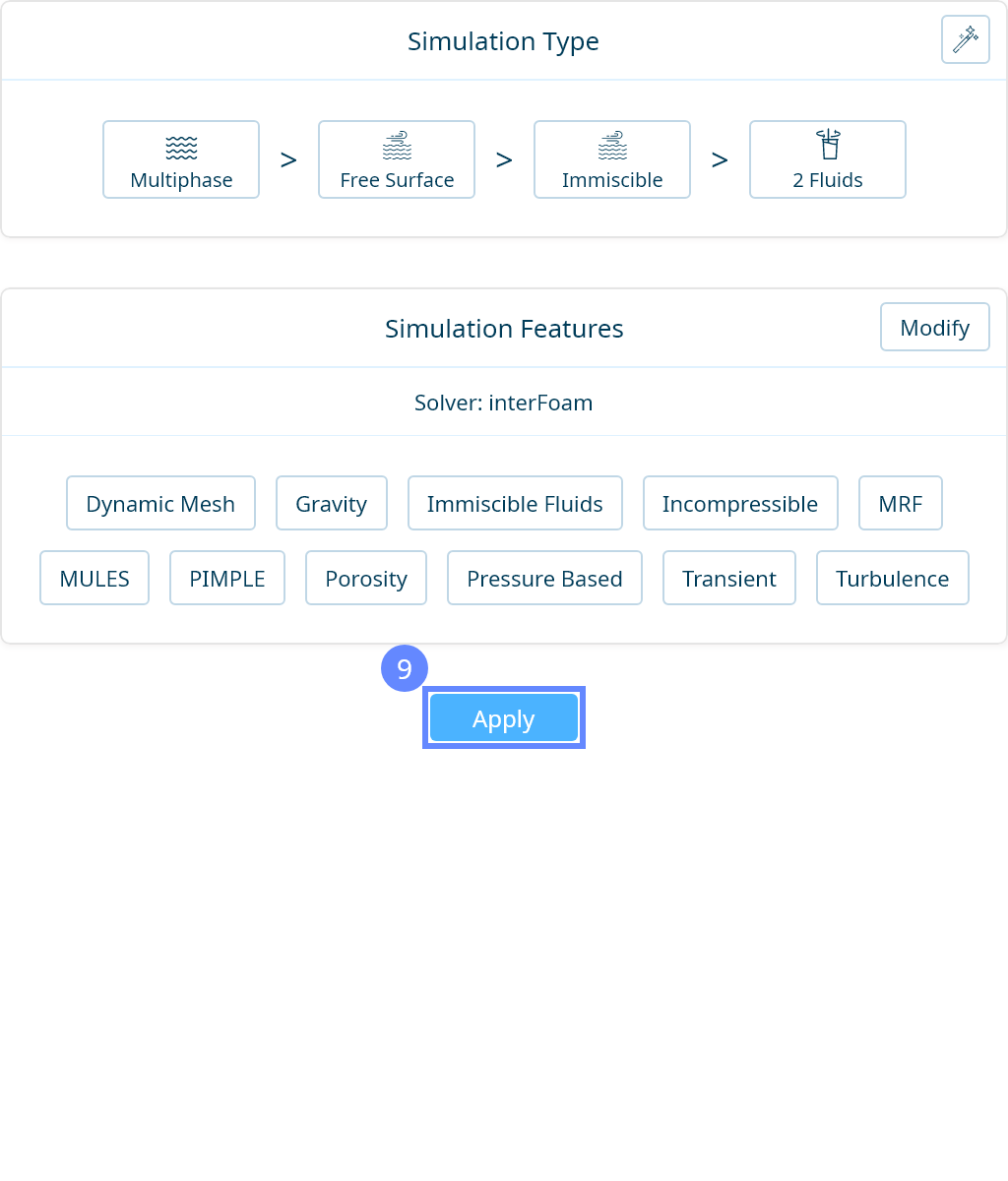
16. Simulation Type
We want to analyze water sloshing in a tank. For this purpose, we will use a transient simulation of two immiscible fluids (water and air) using the free-surface method.

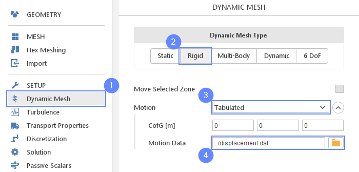
17. Dynamic Mesh
To model tank deceleration we will use a dynamic mesh feature. The dynamic mesh allows transforming mesh by moving its nodes. There are several types of mesh deformation available. In this tutorial, we will use the Rigid type to model mesh translation as a whole.
The external file displacement.dat stores the motion data that we will import to SimFlow. The data describes deceleration from the initial velocity 11.853 m/s to 0 m/s within 5 s .
- Go to Dynamic Mesh panel
- Select Rigid as a Dynamic Mesh Type
- Extend the motion list and select Tabulated
- Indicate the path to the file displacement.dat
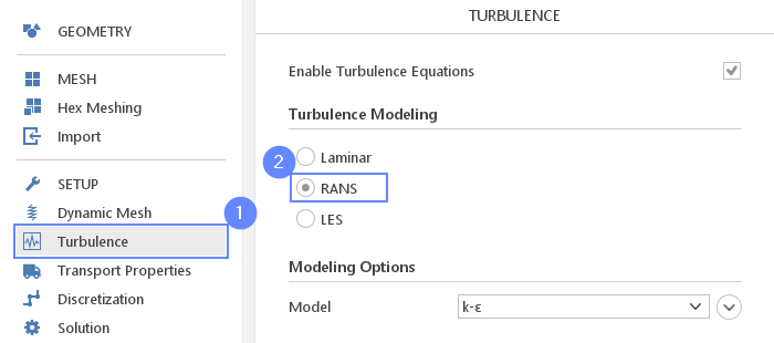
18. Turbulence
In the turbulence panel, enable turbulence modeling and select Raynolds Averaged Navier Stokes (RANS). For the purpose of this tutorial, we will model the turbulence phenomenon using the \(k{-} \varepsilon\) model.
- Go to Turbulence panel
- Set the RANS turbulence formulation
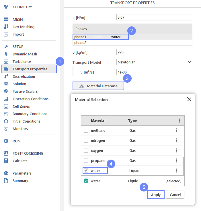
19. Transport Properties - Water
In order to define water and air, we need to go to the transport properties panel, and use predefined fluids properties from the material database.
- Go to
Transport Propertiespanel - Change phase name from
phase1to water - Open Material Database
- Pick up
waterfrom the list - Click Apply
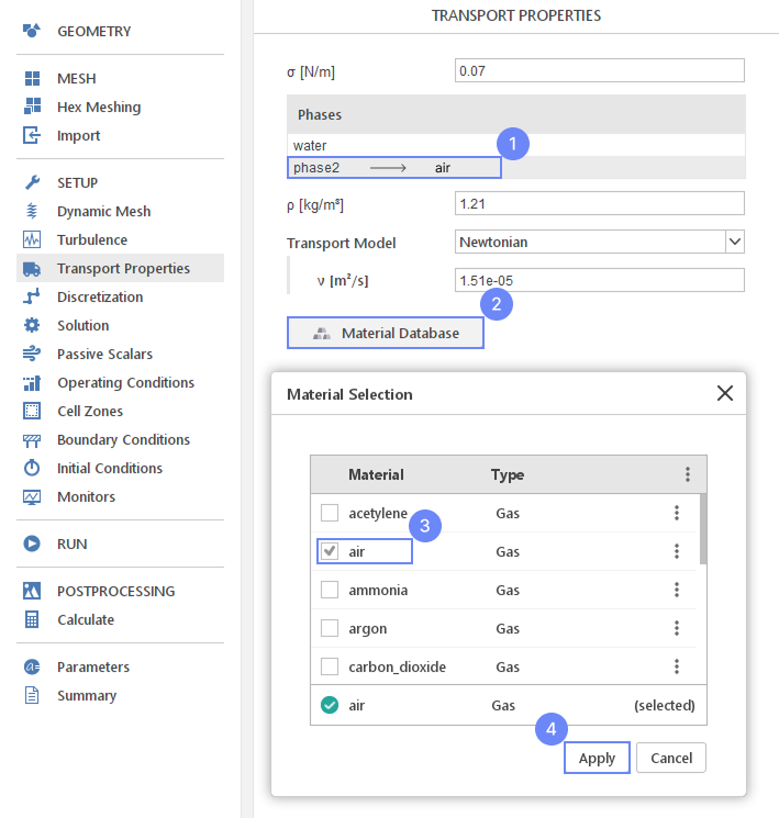
20. Transport Properties - Air
Repeat a previous step for phase2 using air properties.
To assign material to the domain, the phase fraction parameter \(\alpha_{phase}\) is used. The parameter determines the proportion of each fluid in the domain.
The value of phase fraction varies in range from 0 to 1 where \(\alpha_{phase 1}=1\) means that the whole domain is filled only with the phase1, while \(\alpha_{phase 1}=0\) means that the domain is filled with the second phase.
We will assign \(\alpha_{phase}\) parameter in the later steps.
- Rename the second phase
phase2 \(\rightarrow\) air - Verify that the density \(\rho\) and kinematic viscosity \(\nu\) match the correct properties for air
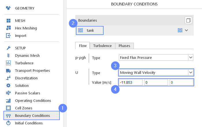
21. Boundary Conditions - Tank (Flow)
The mesh consists of only one tank wall boundary. For this boundary, we will apply the velocity that matches the initial velocity of the tank.
- Go to Boundary Conditions panel
- Select the tank boundary
- 4 Set the velocity type and value accordingly
\(U \quad Type\)Moving Wall Velocity
\(U \quad Value\) \({\sf [m/s]}\)-11.853
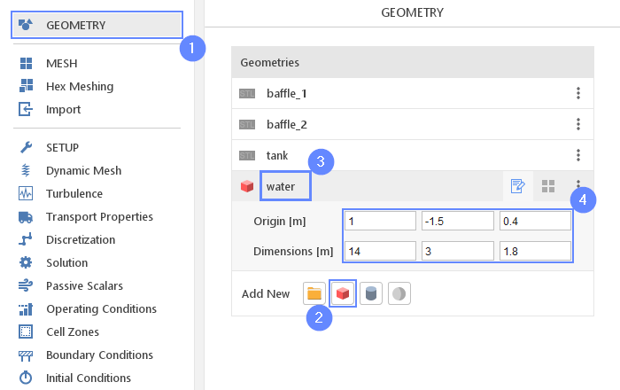
22. Create Geometry - Water
Before we set the initial condition, we need to define the water region. For this purpose, we will create a box that will indicate the initial location of water.
- Go to Geometry panel
- Select Create Box
- Change geometry name from box_1 to water
(double click to edit name and press Enter to confirm) - Expand Properties
- Set the origin and box dimensions
Origin \({\sf [m]}\)1-1.50.4
Dimensions \({\sf [m]}\)1431.8
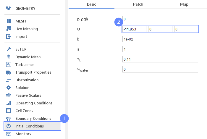
23. Initial Conditions - Basic
Before we start the calculation, we need to define the fluid state at the time zero. We will specify the velocity to be equal to -11.853 m/s which corresponds to the initial tank velocity.
To assign the material to the domain, the phase fraction parameter \(\alpha_{phase}\) is used. The parameter determines the proportion of each fluid in the given point in space. The phase fraction value varies in range from 0 to 1, where \(alpha_{phase1}=1\) denotes phase1, while \(alpha_{phase1}=0\) denotes remaining fluid - the second phase.
At the initial state, a water phase fraction is equal to \(\alpha_{water} =0\) which means that the whole domain is filled with air by default. In the next step we will patch a bottom region by the water.
- Go to Initial Conditions panel
- Set the initial velocity
U-11.85300
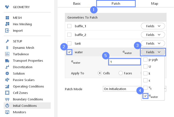
24. Initial Conditions - Patch
Using the water geometry, we will overwrite the phase fraction value inside it. We will set the \(\alpha_{water}\) to 1 to fill the patched geometry with water.
- Switch to Patch tab
- Check the water geometry
- Expand the Fields
- Check \(\alpha_{water}\)
- Set initial value of \(\alpha_{water}\) to 1
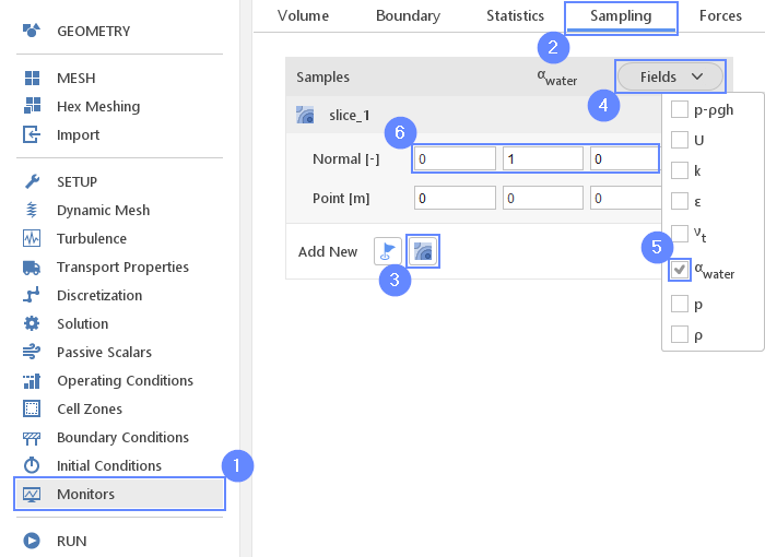
25. Monitors - Create Slice
During calculation, we can observe intermediate results on a section plane. To add sampling data on a plane, we need to define plane properties and also select variables that will be sampled. Note that runtime post-processing can only be defined before starting calculations and cannot be changed later on.
- Go to Monitors panel
- Switch to Sampling tab
- Select Create Slice
- Expand Fields list
- Select the water phase \(\alpha_{water}\)
- Set the normal along Y axis
Normal \({\sf [-]}\)010
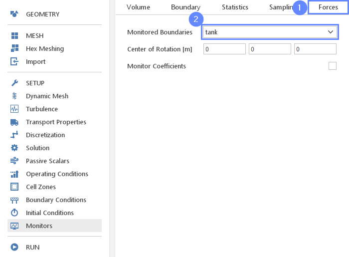
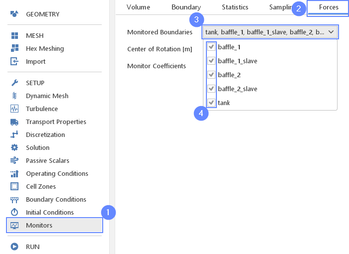
26. Monitors - Forces
In order to track the sloshing force on the tank boundary, we will use the force monitor.
- Switch to Forces tab
- Expand Monitored Boundaries list and check tank
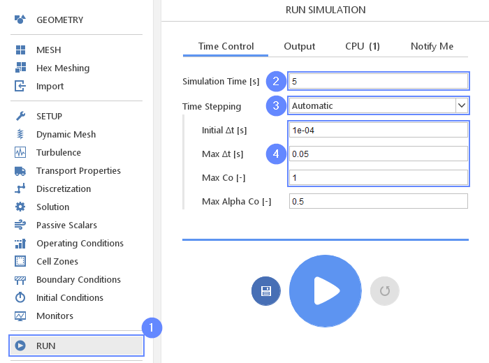
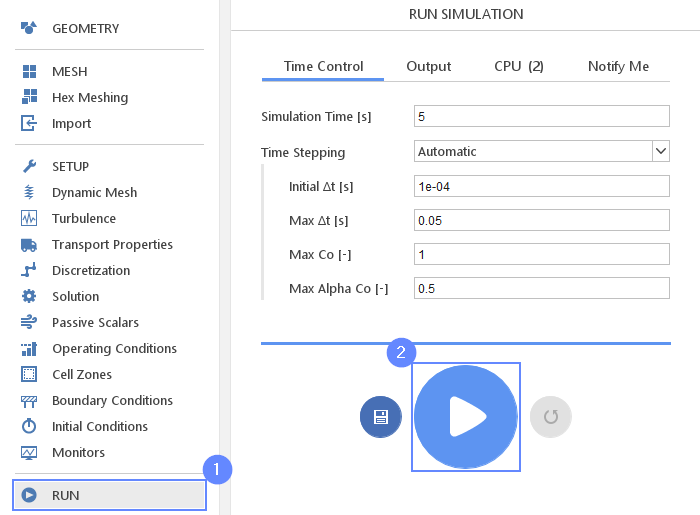
27. Run - Time Control
For any simulation, it is very convenient to let the solver automatically determine the proper time step value. To use this option, we need to define time step constraints by providing the initial time step (adjusted by the solver during computations), maximal time step value and Courant number.
- Go to RUN panel
- Set the Simulation Time [s] to 5
- Change Time Stepping to Automatic
- Set initial time step, maximum time step and Courant number accordingly
Initial \(\Delta t\) \({\sf [s]}\)1e-04
(solver will start computation with this value and adjust it in the next iterations)
Max \(\Delta t\) \({\sf [s]}\)0.05
Max Co \({\sf [-]}\)1
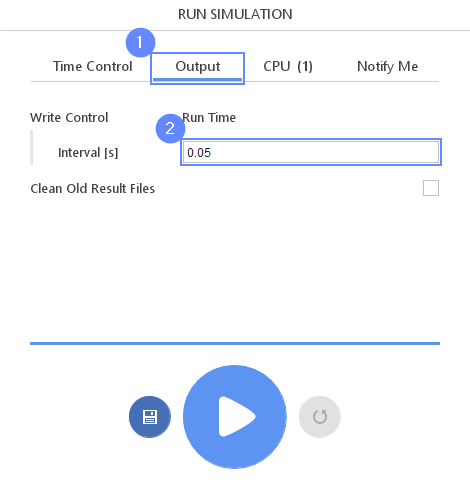
28. Run - Output
We can control how often results should be saved on the hard drive. Only this data will be available for postprocessing.
- Switch to Output tab
- Set the Interval [s] to 0.05
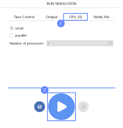
29. Run - CPU
To speed up the calculation process, take advantage of parallel computing and increase the number of CPUs based on your PC’s capability. The free version allows you to use only one processor (serial mode). To get the full version, you can use the contact form to Request 30-day Trial
Estimated computation time for serial mode: 1,5 hours
- Switch to CPU tab
- Click Run Simulation button
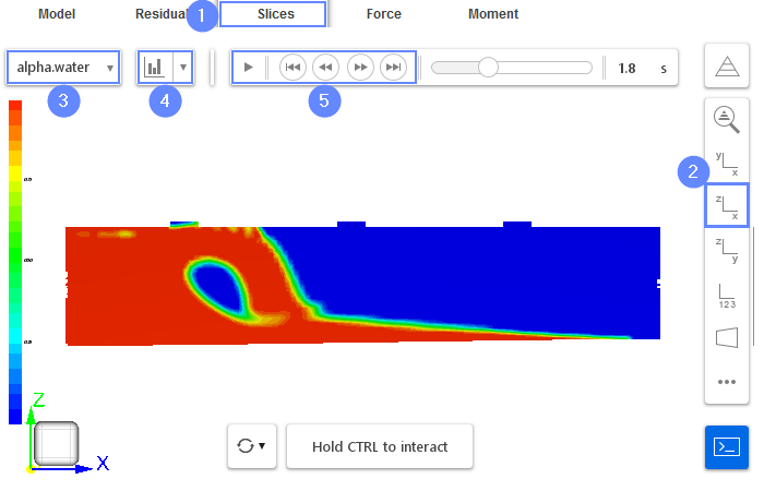
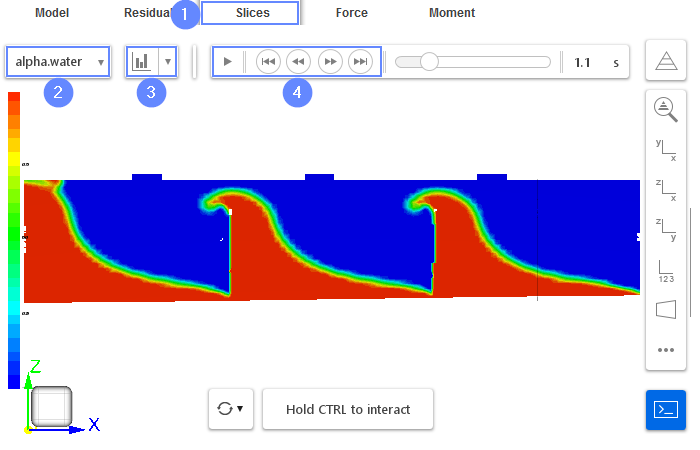
30. Results - Slice
Slices tab appears next to Residuals. Under this tab, we can preview results on the defined slice planes. The results preview is available during the calculation and we can track it on a regular basis. The newly calculated time step will be actualized automatically as long as the time selector points to the latest time step.
- Change tab to Slice
- Set the View XZ
- Choose alpha.water field to display the water phase
- Click Adjust range to data
- Play with animation buttons to view the results of the analysis
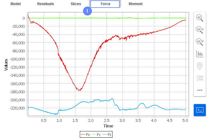
31. Results - Force
Additional force tab appears next to Slices . Under this tab, we can view force plots. The results preview is available during the calculation and we can use it to track the progress of the simulation as well.
- Change tab to Force
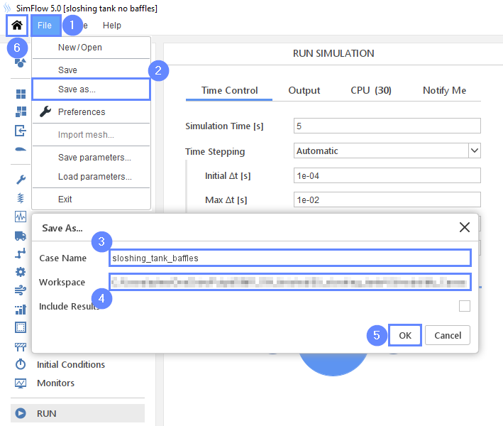
32. Save model
We will use this simulation as a starting point for the second configuration. To do so, we will save the current model under a new name without the results.
- Extend File options from the top menu
- Select Save as…
- Type new name sloshing_tank_baffles
- The model will be saved in the same location by default
- Press OK
- Go to Launcher
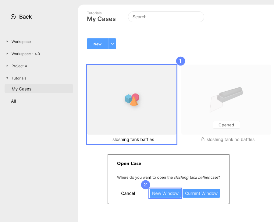
33. Load model
After saving, we will open a new case.
- Select a case sloshing tank baffles from launcher
- Open the case in New Window
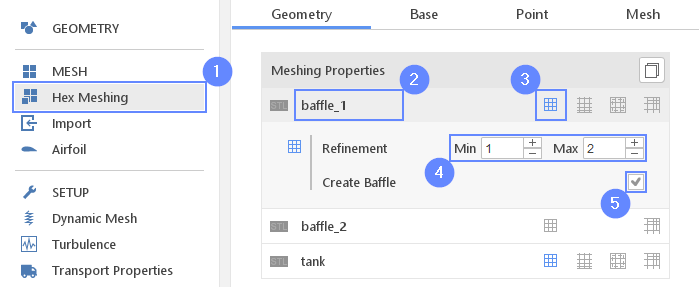
34. Meshing Parameters - Baffle 1
In the new case, we will add the baffles inside the tank. The baffles geometries are already loaded in SimFlow but have not been used yet. We can just turn them on and remesh the model.
- Go to Hex Meshing panel
- Select the baffle_1
- Enable Mesh Geometry
- Set Refinement to Min 1 Max 2
- Check Create Baffle option
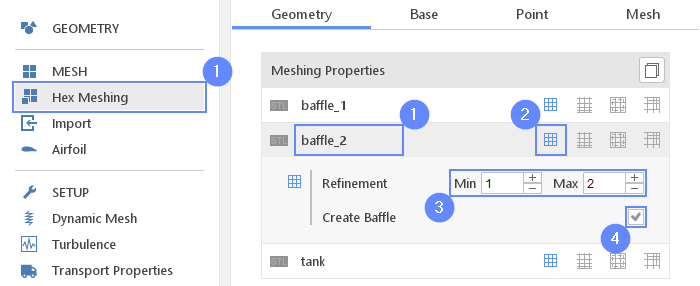
35. Meshing Parameters - Baffle 2
Repeat these steps for the second baffle.
- Select the baffle_2
- Enable Mesh Geometry
- Set Refinement to Min 1 Max 2
- Check Create Baffle option
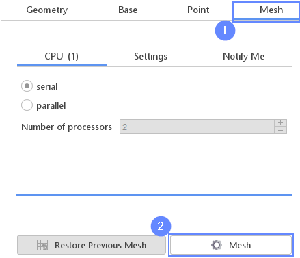
36. Start Meshing - Second Case
We will use the same base mesh setup so we can go directly to the meshing step.
- Go to Mesh tab
- Press the Mesh button to start meshing process
37. Boundary Conditions - Copy (I)
We have already defined the initial velocity of the tank. Now, we need to assign the velocities to the remaining walls. We will copy the boundary conditions from the tank to the others.
- Go to Boundary Conditions panel
- Select the tank boundary

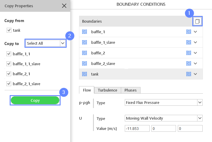
38. Boundary Conditions - Copy (II)
- Press Copy Boundary Conditions
- Extend the list next to Copy to and press Select All . All boundaries will be checked
- Press Copy
39. Monitors - Forces (2nd Case)
Previously fluid was acting only on the tank boundary. In the current mesh, we have additional walls that should participate in force calculation as well.
- Go to Monitors panel
- Switch to Forces tab
- Expand the list of Monitored Boundaries
- Check all boundaries
40. Run Second Case
Finally, we can run the simulation using the same parameters as previously.
- Go to RUN panel
- Click Run Simulation button
41. Results - Slice (2nd Case)
We can view the results on the slice.
- Switch to Slice tab
- Select alpha.water field to display the water phase
- Click Adjust range to data
- Play with animation buttons to view the results of the analysis
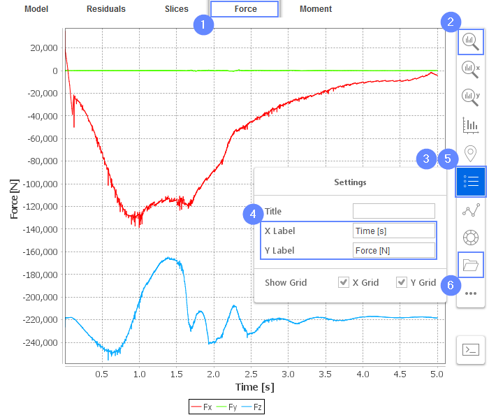
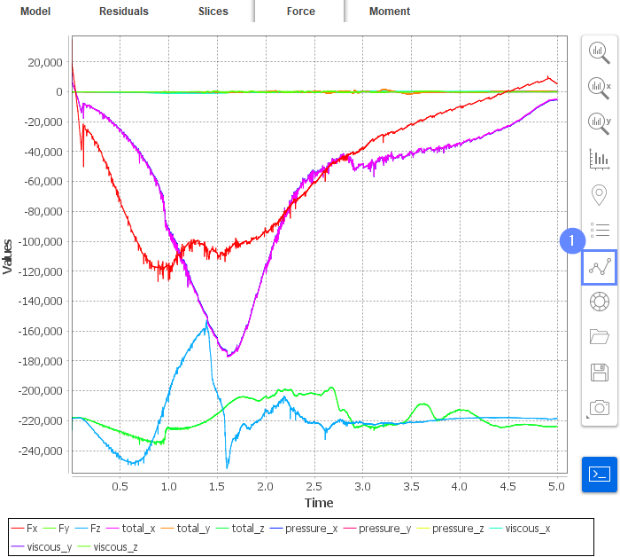
42. Results - Force (2nd Case)
Under the force tab, we will display the resultant force acting on a tank caused by fluid deceleration. We will add the results from the previous simulation (without the baffles) and compare them on the same chart.
- Change tab to Force
- Click on Fit Axes
- Click on Chart Setup
- Set the name of the axis:
X Label to Time [s]
Y Label to Force [N] - To close the panel press Chart Setup button once again or press Esc key
- Clisk Plot Data from File button
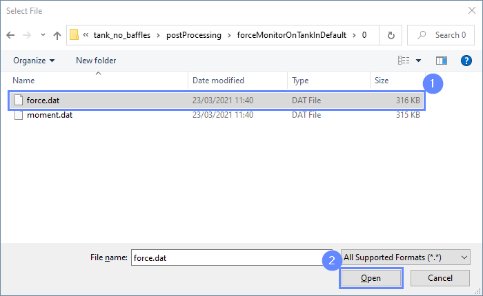
43. Import Results
- Navigate to the folder with a previous simulation sloshing_tank_no_baffles . The forces were automatically saved under the following path
…/sloshing_tank_no_baffles/postProcessing/forceCompositeMonitorOnTankInDefault/0 - Select the file force.dat
- Press Open
44. Results Summary
New data series will be added to the chart. We will hide the unnecessary data series for clarity.
- Select Data Series
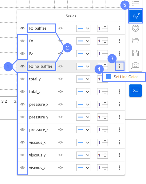
45. Results - Data Series
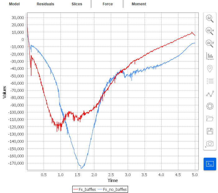
We will leave only the sloshing force (force along X direction).
- Hide all series except Fx and total_x
- Change series name accordingly
Fx \(\rightarrow\) Fx_baffles
total_x \(\rightarrow\) Fx_no_baffles - Click on Options next to Fx_no_baffles
- Set the color of the series to blue
- Click Data Series to exit or press Esc key
46. Results Comparison
Finally, we can compare the results from both configurations. We can see that the peak force was reduced by 30% by using baffles.