3. Create Case
Open SimFlow and create a new case named spray combustion
- Click New
- Provide name spray combustion
- Click Create to open a new case

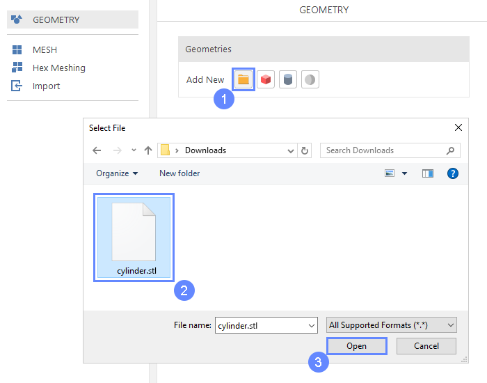
4. Import Geometry
Firstly we need to Download GeometryCylinder
- Click Import Geometry
- Select geometry file cylinder.stl
- Click Open
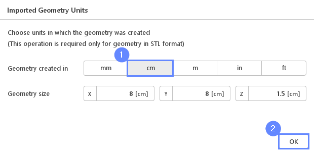
5. Imported Geometry Units
The STL format does not contain the unit information which are defined during the geometry export. If we do not know the exported unit, we can estimate it based on the total size of the model. It is displayed next to Geometry size label. In our case, the default unit meter is correct.
- Select cm unit
- Click OK button
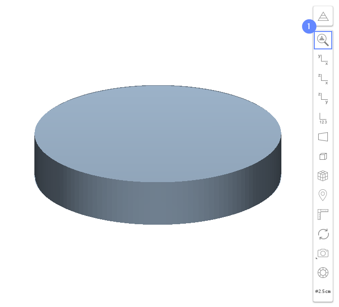
6. Geometry - Cylinder
After importing geometry, it will appear in the 3D window.
- Click Fit View to zoom in on the geometry.
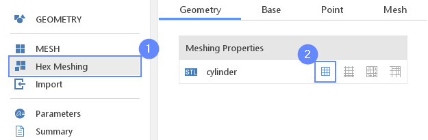
7. Meshing Parameters - Cylinder
In order to create the mesh, we need to enable meshing for the newly imported geometry.
- Go to Hex Meshing panel
- Enable Mesh Geometry on cylinder geometry
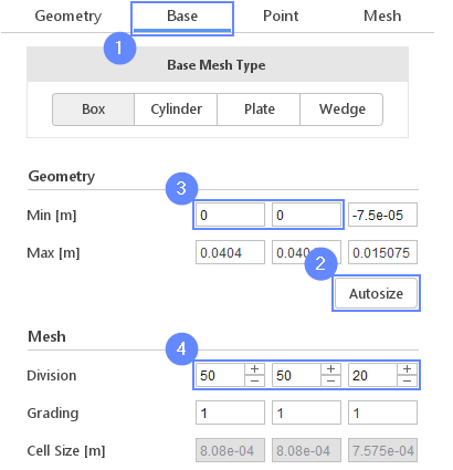
8. Base Mesh - Domain
Now we will define the base mesh. The box geometry determines the background mesh domain. The model is symmetrical on the XZ and YZ planes so we do not need to mesh the whole geometry. Using the box dimensions we will choose only a quarter of a model.
- Switch to Base tab
- Click on Autosize
- Change the following parameters accordingly
Min \({\sf [m]}\)00 - Define the number of divisions
Division505020
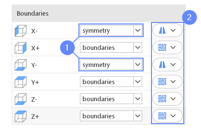
9. Base Mesh - Boundaries
We need to assign individual names to each side of the base mesh. This will allow us to apply different conditions to each side.
- Change the following boundary names
X- symmetry
Y- symmetry - Set the types for boundaries accordingly
X- symmetry
X+ wall
Y- symmetry
Y+ wall
Z- wall
Z+ wall
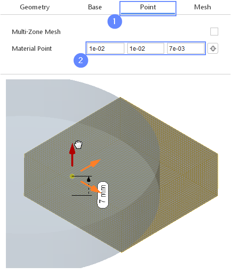
10. Material Point
Material Point tells the meshing algorithm on which side of the geometry the mesh is to be retained. Since we are considering flow inside the cylinder, we need to place the material point inside the geometry.
- Switch to Point tab
- Specify location inside the cylinder
Material Point1e-021e-027e-03
You can specify the point location from the 3D view. Hold the CTRL key and drag the arrows to the destination.
11. Start Meshing
- Go to Mesh tab
- Start the meshing process with Mesh button
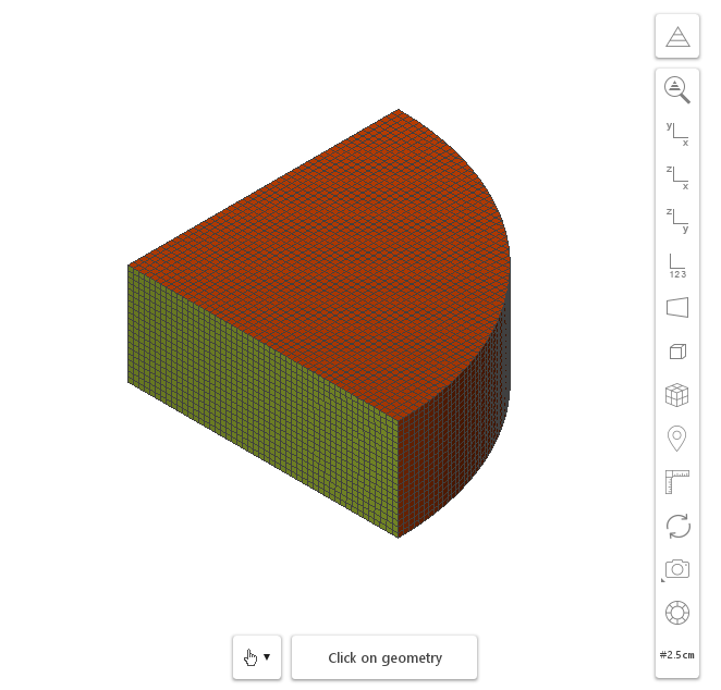
12. Examine Mesh
After the meshing process is complete, the mesh should appear in the graphics window. To zoom in or zoom out use the scroll wheel , or move the mouse up or down with pressed RMB (right mouse button).
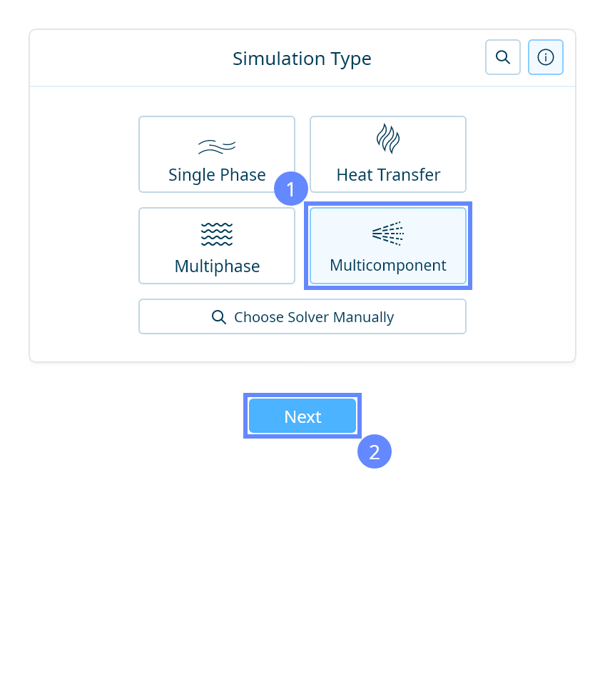
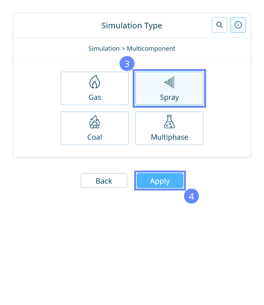
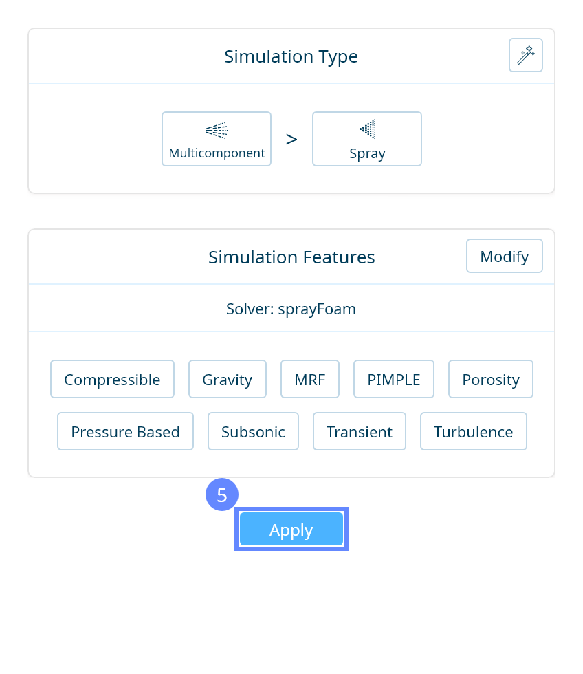
13. Simulation Type
We want to analyze spray combustion inside a cylinder. For this purpose, we will use a transient simulation with species transport, combustion and Lagrangian spray particles.

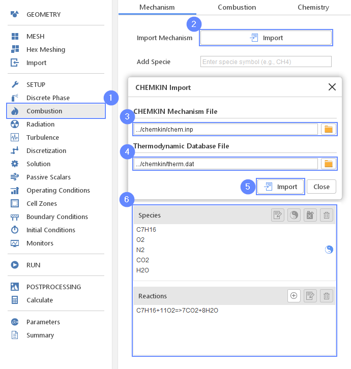
14. Combustion - Mechanism
We will load the chemical kinetic mechanism as well as the thermodynamic properties database. We will consider only the one chemical reaction describing the process which is a simplification in order to decrease the computational cost and calculation time.
To complete this step we need to Download Fileschem.inptherm.dat
After that, import them to the SimFlow.
- Go to Combustion panel
- Click Import mechanism
- For CHEMKIN Mechanism File select the chem.inp
- For Thermodynamic Database File select the therm.dat
- Click Import
- Check and validate the listed Species and Reactions
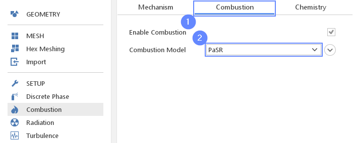
15. Combustion - Model
We will select the partially stirred reactor model which is used to simulate combustion.
- Switch to Combustion tab
- Select Combustion Model as a PaSR
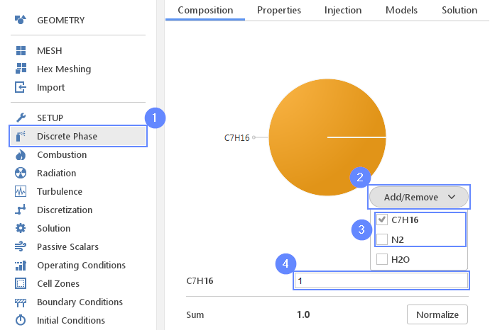
16. Discrete Phase - Composition
We will select the pure heptane as a phase injected into the chamber.
- Go to Discrete Phase panel
- Extend Add/Remove list
- Check C7H16 phase and uncheck N2 phase
- Set the C7H16 mass fraction to 1
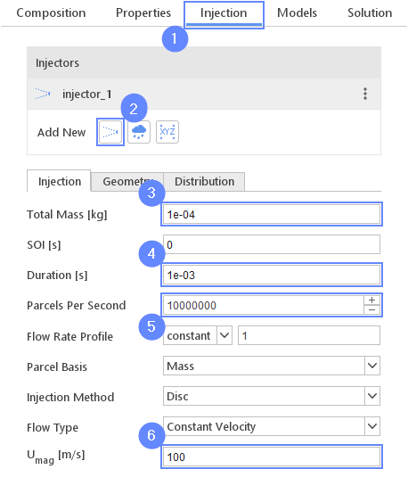
17. Discrete Phase - Injection
We are going to create a cone injector and define its parameters.
- Switch to Injection tab
- Add new Cone Injector
- Set Total Mass [kg] injection to 1e-04
- Set Duration [s] injection to 1e-03
- Set Parcels Per Second to 10000000
- Set the velocity \(U_{mag} \; [m/s]\) to 100
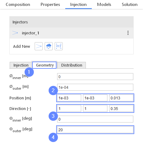
18. Discrete Phase - Injection Geometry
We need to define the position of the injector and spray outflow direction.
- Go to Geometry tab
- Set the position of injector
Position \({\sf [m]}\)1e-031e-030.013 - Set the injection direction
Direction \({\sf [-]}\)110.35 - Set the outer cone angle \(\Theta_{outer} \; [deg]\) to 20
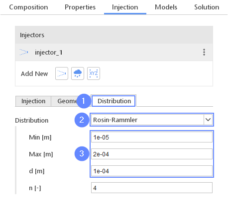
19. Discrete Phase - Injection Distribution
We will select the Rosin-Rammler distribution model and define the necessary parameters. Models need to define the minimum and maximum spray droplet diameter and size which is the largest probability.
- Switch to Distribution tab
- Select the Rosin-Rammler model from drop down list
- Set the minimal, maximal and nominal droplet diameter:
Min \({\sf [m]}\)1e-05
Max \({\sf [m]}\)2e-04
d \({\sf [m]}\)1e-04
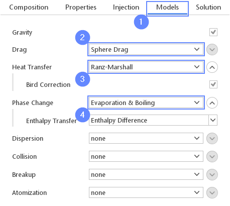
20. Discrete Phase - Models
We need to define which models will be used in this simulation. We select the Sphere Drag model to account for the drag force acting on the droplets. We choose the Ranz-Marshall heat transfer model to take into account heat transfer between the spray droplets and surrounding gas. For accounting mass transfer from the droplets to the gas as a result of the evaporation and boiling we use the Evaporation & Boiling model.
- Switch to Models tab
- Set the drag model as Sphare Drag
- Set the heat transfer model as Ranz-Marshall
- Set the drag model as Evaporation & Boiling
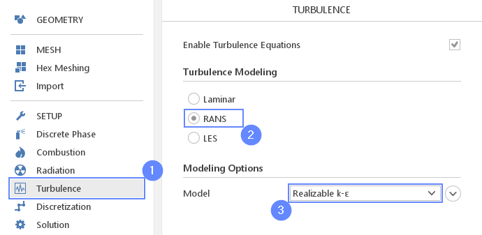
21. Turbulence
For the purpose of this tutorial, we will simulate the turbulence phenomenon using the Realizable \(k {-} \varepsilon\) model.
- Go to Turbulence panel
- Select RANS turbulence formulation
- Select Realizable \(k {-} \varepsilon\) model
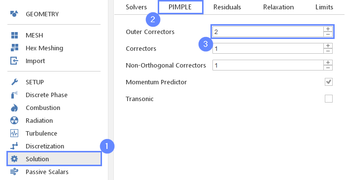
22. Solution - PIMPLE
To increase the stability of the simulation we will increase the number of iterations per time step.
- Go to Solution panel
- Switch to the PIMPLE tab
- Set Outer Correctors to 2
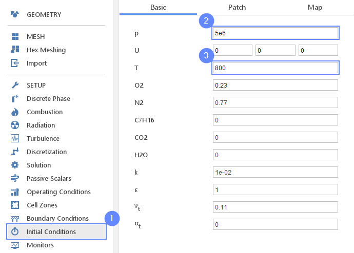
23. Initial Conditions - Basic
Initially, the entire domain is filled with air. We will set the initial pressure and temperature in the chamber.
- Go to Initial Conditions panel
- Set the initial pressure in the chamber P to 5e6 Pa
- Set the initial temperature in the chamber T to 800 Kelvin
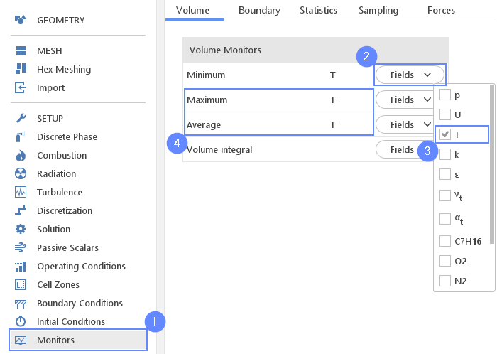
24. Monitors - Temperature
In order to measure maximum and minimum temperature, we will use the volume monitor.
- Go to Monitors panel
- Expand the Fields for the Minimum volume monitors
- Select the temperature field T
- Repeat this step for the Maximum and Average volume monitors.
Selected fields will be visible next to the volume monitor names.
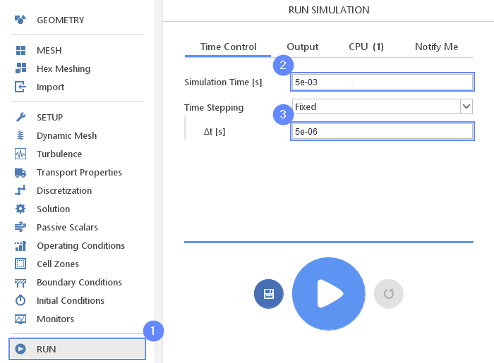
25. Run - Time Control
Before running computations, adjust the time controls in order to capture the physical and chemical phenomena that occur during the process.
- Go to RUN panel
- Set the Simulation Time [s] to 5e-03
- Set the Time Stepping \(\Delta \sf{t[s]}\) to 5e-06
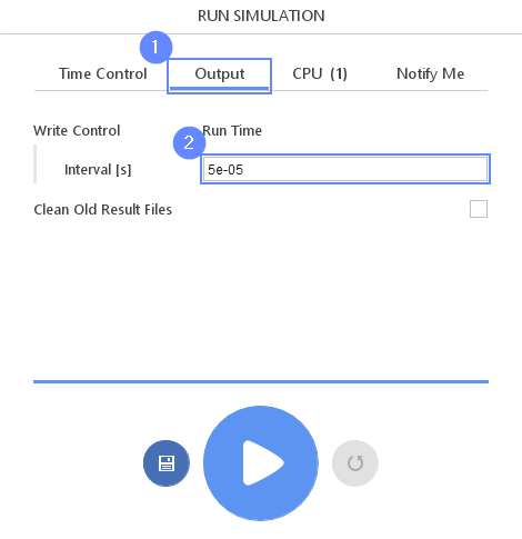
26. Run - Output
We can control how often results should be saved on the hard drive. We will write the results at the interval of \(5e-05\) second. Note, that only saved data will be available during postprocessing.
- Switch to Output tab
- Set the Interval [s] to 5e-05
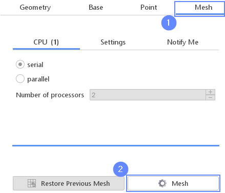
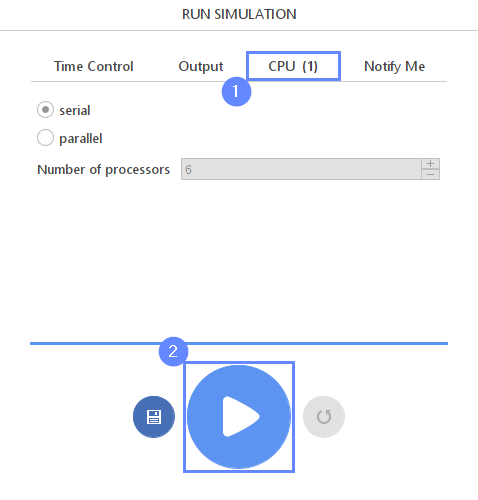
27. Run - CPU
To speed up the calculation process, take advantage of parallel computing and increase the number of CPUs based on your PC’s capability. The free version allows you to use only one processor (serial mode). To get the full version, you can use the contact form to Request 30-day Trial
Estimated computation time for serial mode: 3 hours
- Switch to CPU tab
- Click Run Simulation button
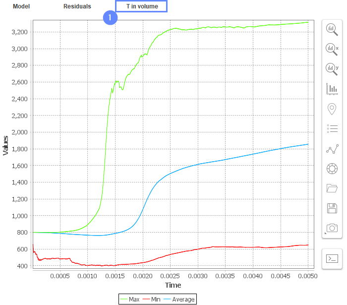
28. Results - Temperature
Keep track of the domain’s maximum and minimum temperature. A sudden increase in temperature is a result of the combustion process.
- Switch tab to T in volume next to the residuals
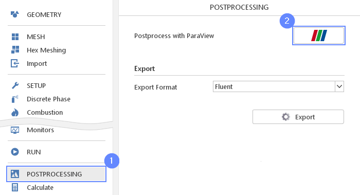
29. Postprocessing - ParaView
After the computation is finished we can do a comprehensive visualization of our results with ParaView.
- Go to POSTPROCESSING panel
- Click on Run ParaView
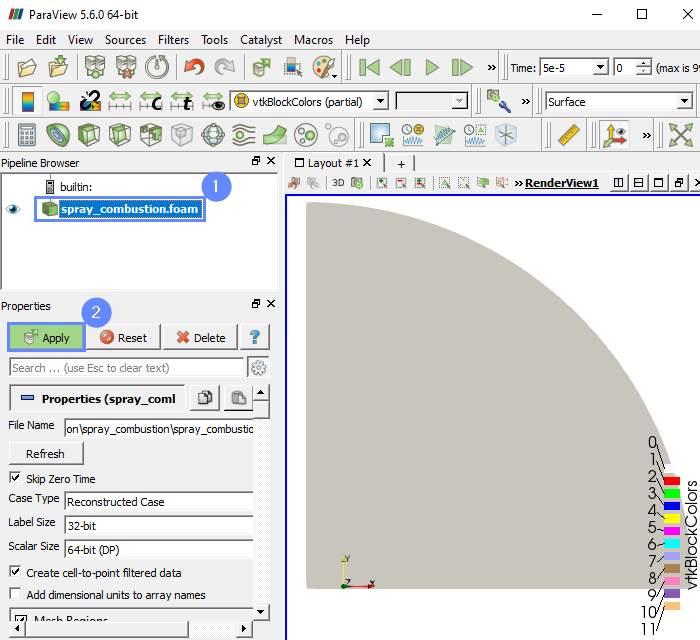
30. ParaView - Load Results (I)
Load the results into the program.
- Select spray_combustion.foam
- Click Apply to load results into ParaView
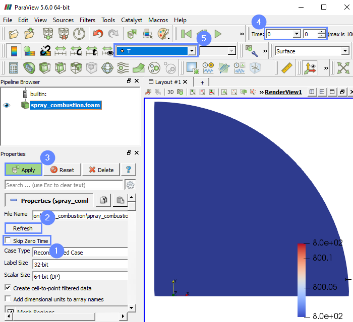
31. ParaView - Load Results (II)
ParaView skips the initial time step by default, therefore we need to add the zero time to simulation.
- Uncheck Skip Zero Time
- Click Refresh
- Click Apply
- Set the time or time step to 0
- Select temperature T
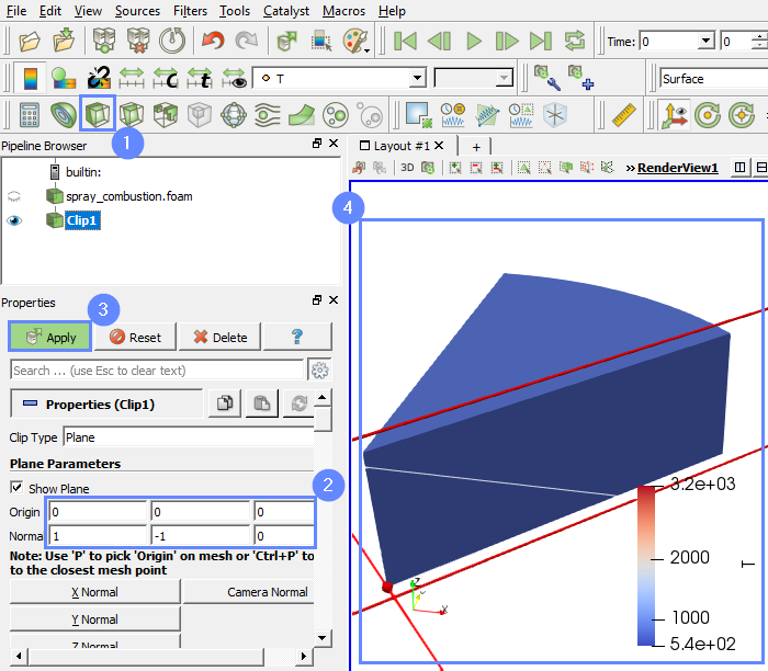
32. ParaView - Clip
We will slice the domain in the direction of spray combustion.
- Select Clip options from top menu
- Define the origin and normal of the clip plane:
Origin000
Normal1-10 - Click Apply
- Check the clip in the 3D graphic window
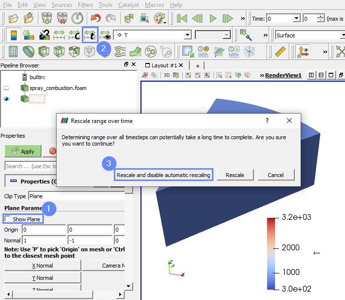
33. ParaView - Temperature (I)
Now we will check the temperature distribution during the process.
- Uncheck Show Plane for better visualisation
- Select Rescale to data range over all timesteps
- Confirm choise by clicking Rescale and disable auromatic rescaling
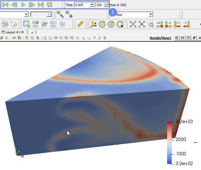
34. ParaView - Temperature (II)
- Play with animation buttons to track the results of the analysis.
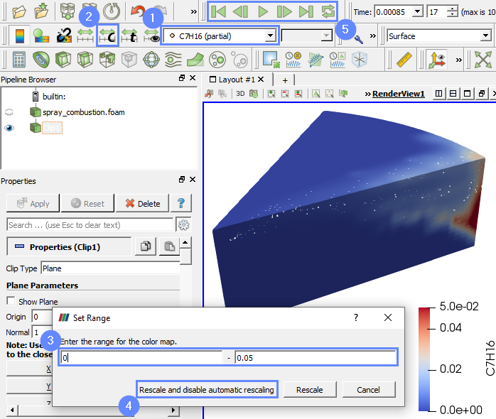
35. ParaView - Spray Phase
Finally, we will look at the spray particle movement.
- Select C7H16 (partial) from the list
- Click Rescale to Custom Data Range
- Set the range from 0 to 0.1
- Confirm by clicking Rescale and disable automatic rescaling
- Play with an animation buttons to track the results of analysis.