3. Create Case
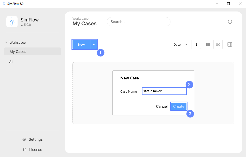
Open SimFlow and create a new case named static mixer
- Click New
- Provide name static mixer
- Click Create to open a new case
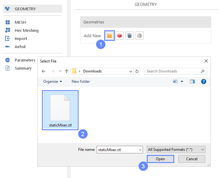
4. Import Geometry
Firstly we need to Download GeometryStaticMixer
- Click Import Geometry
- Select geometry file staticMixer.stl
- Click Open
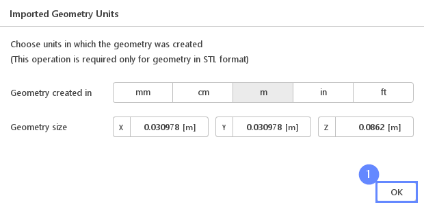
5. Imported Geometry Units
The STL format does not contain the unit information which are defined during the geometry export. If we do not know the exported unit, we can estimate it based on the total size of the model. It is displayed next to Geometry size label. In our case, the default unit meter is correct.
- To confirm default unit meter, press OK
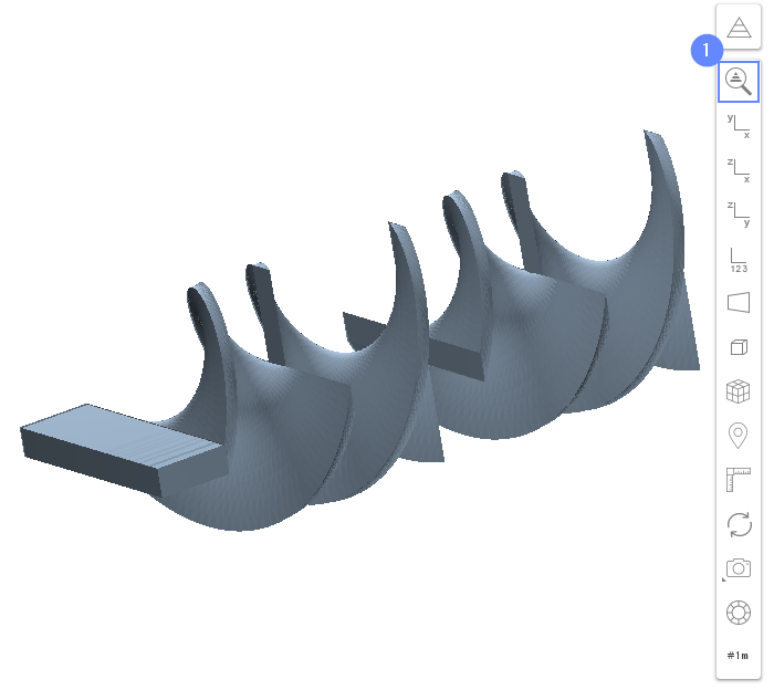
6. Geometry - Static Mixer
After importing geometry, it will appear in the 3D window.
- Click Fit View to zoom in on the geometry.
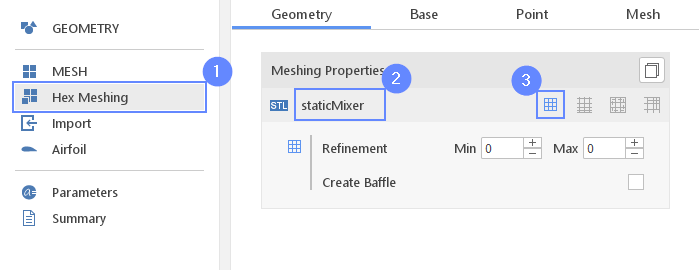
7. Meshing Parameters - Static Mixer
In order to create the mesh, we need to enable meshing for the imported geometry.
- Go to Hex Meshing panel
- Select staticMixer geometry
- Enable Mesh Geometry
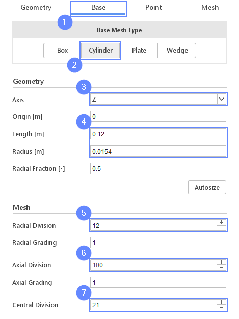
8. Base Mesh - Domain
The imported geometry represents only the mixer blades. By using a cylinder base mesh we will define the pipe housing.
- Switch to Base tab
- Choose base mesh type
Base Mesh Type Cylinder - Set the cylinder axis
Axis Z - Set the size of the cylinder base mesh:
Length \({\sf [m]}\)0.12
Radius \({\sf [m]}\)0.0154 - 67 Set the following parameters accordingly
Radial Division12
Axial Division100
Central Division21
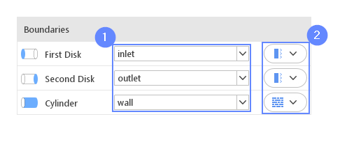
9. Base Mesh - Boundaries
We need to assign individual names to each side of the base mesh. This will allow us to apply different conditions to each side.
- Choose boundary names accordingly
First Disk inlet
Second Disk outlet
Cylinder type wall in the text box
To edit a name: place the cursor to modify text, or double-click to select and overwrite text. Adding a new name will automatically save it to the list. - Choose boundary types accordingly
First Disk patch
Second Disk patch
Cylinder wall
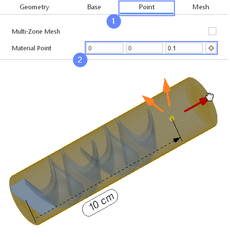
10. Material Point
Material Point tells the meshing algorithm on which side of the geometry the mesh is to be retained. Since we are considering flow inside the cylinder we need to place the material point outside the blades.
- Switch to Point tab
- Specify the location of the material point inside staticMixer
Material Point000.1
You can specify the point location from the 3D view. Hold the CTRL key and drag the arrows to the destination.
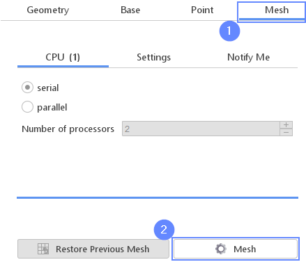
11. Start Meshing
- Go to Mesh tab
- Start the meshing process with Mesh button
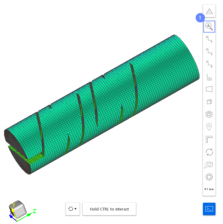
12. Mesh
After the meshing process is finished the mesh should appear in the graphics window.
- Click Fit View to zoom in the mesh
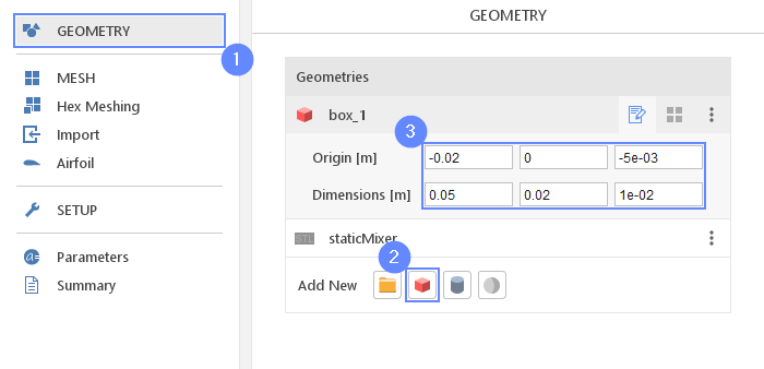
13. Create Geometry - Box
To provide two different fluids into the mixer, we need to split the inlet boundary into two separate ones. We will use additional geometry to mark the selection for the extraction.
- Go to Geometry panel
- Select Create Box
- Set the origin and box dimensions
Origin \({\sf [m]}\)-0.020-5e-03
Dimensions \({\sf [m]}\)0.050.021e-02
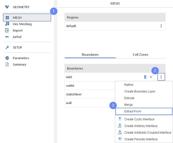
14. Inlet Boundary (I)
Now, using the new geometry we will extract a new boundary from the original inlet.
- Go to MESH panel
- Expand the Options list next to inlet boundary
- Select Extract From option
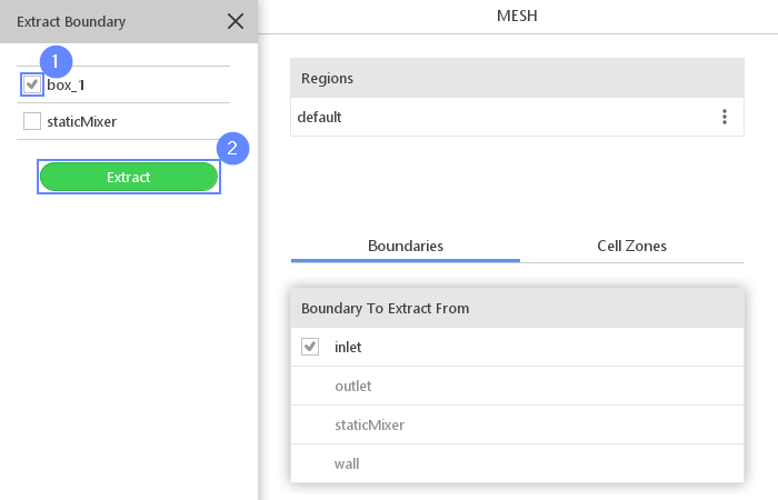
15. Inlet Boundary (II)
- Check box_1
- Click Extract
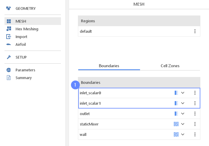
16. Inlet Boundary (III)
- Change the names accordingly
inlet → inlet_scalar0
inlet_in_box_1 → inlet_scalar1
(double click on the name to change it)
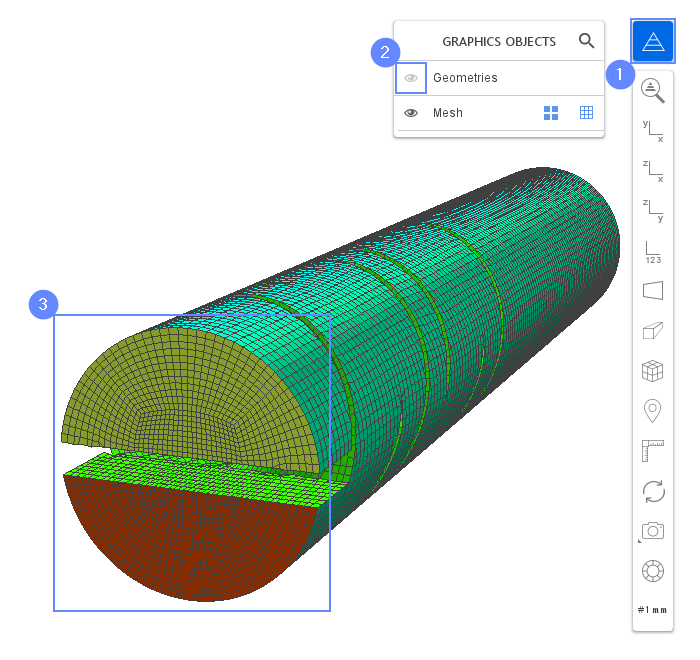
17. Inlet Boundary (IV)
As the results of the extraction, we should receive two separate inlet boundaries. Both boundaries can be distinguished by the different colors.
- Expand Graphics Objects List
- Uncheck the icon next to the Geometries to hide all geometry and press the Esc key
- Check if the inlet boundaries are colored differently
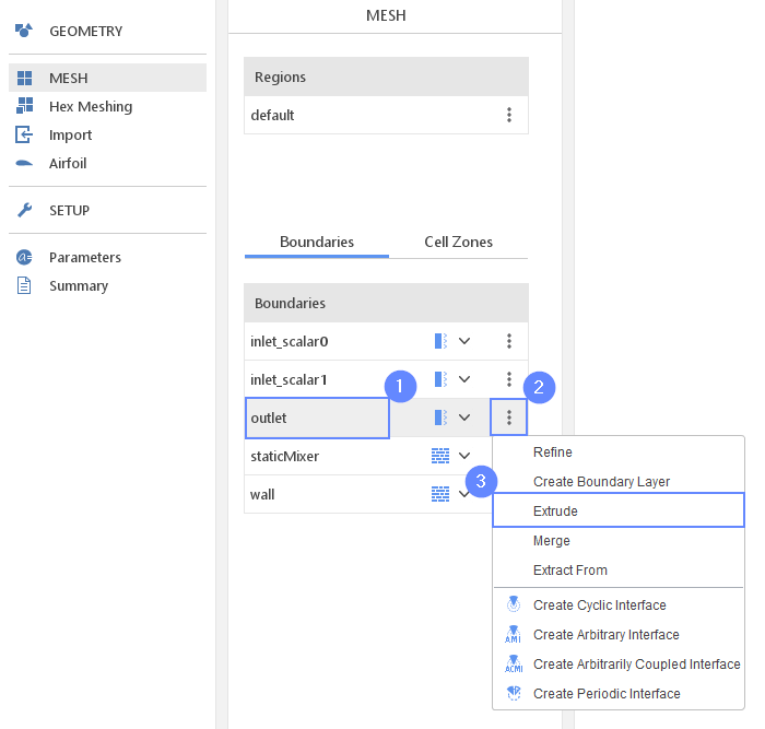
18. Domain Modification (I)
With SimFlow, the user can also modify the existing mesh domain. We can extend the volume by extruding a specific boundary. For the purpose of this tutorial, we will extend the mixer tube by extruding the outflow face.
- Select outlet boundary
- Expand the Options list
- Select Extrude option
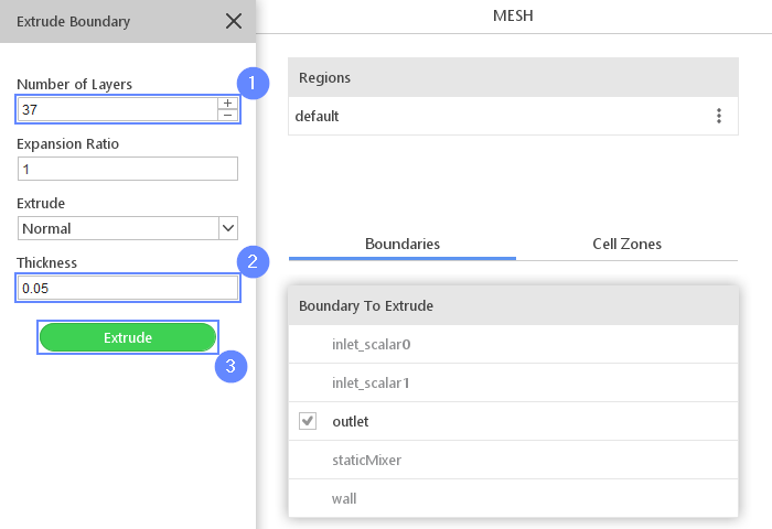
19. Domain Modification (II)
The outlet boundary will be extended by 5 cm and additional mesh will be split into 37 cells in the extrusion direction.
- Set the layer’s number accordingly
Number of Layers37 - Set the thickness accordingly
Thickness0.05 - Click Extrude
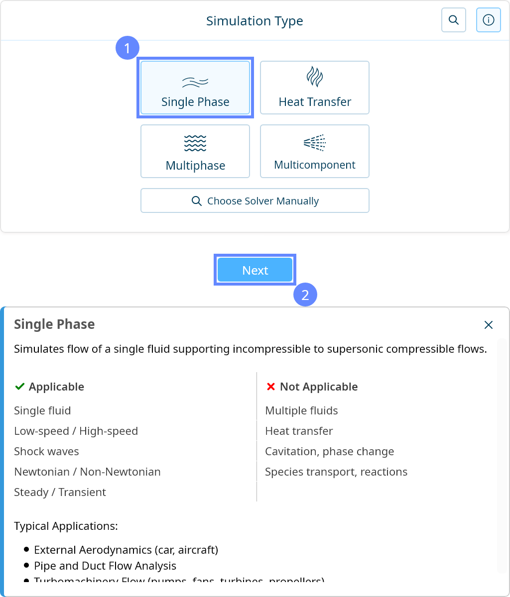
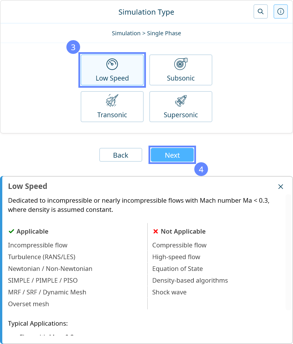
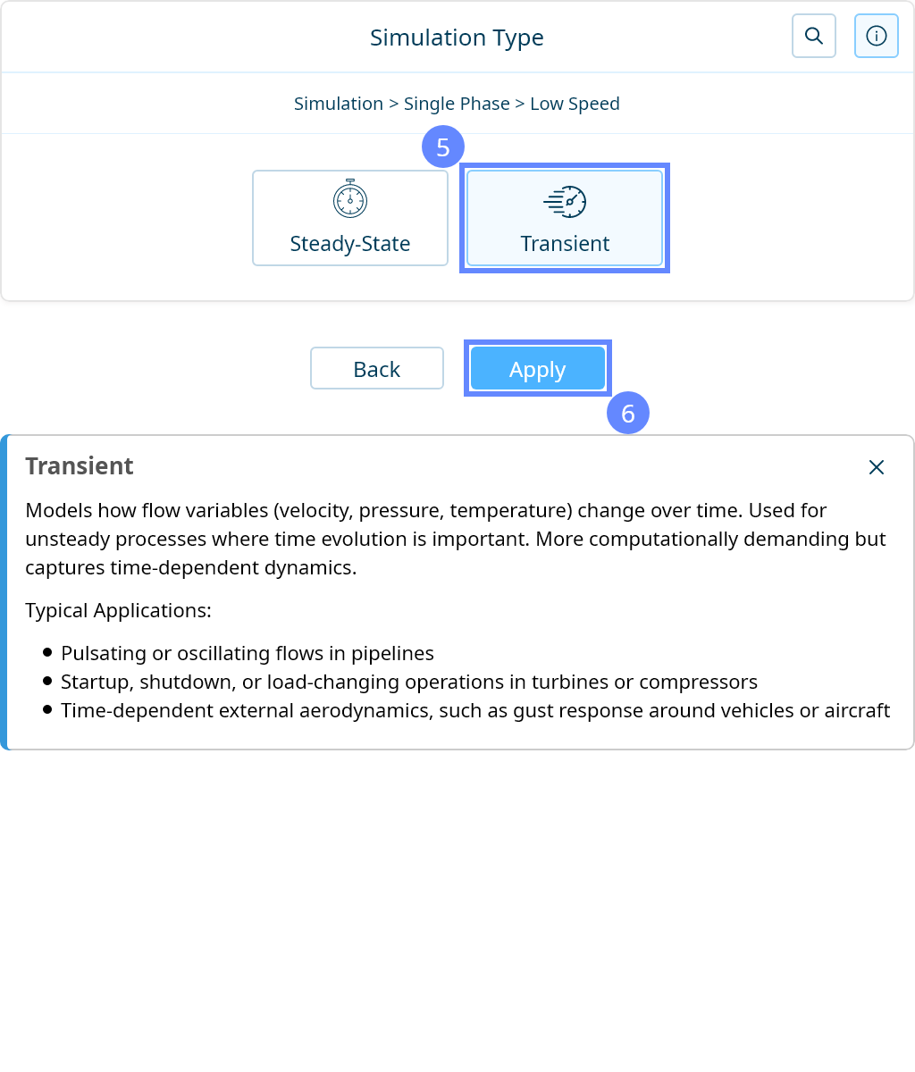
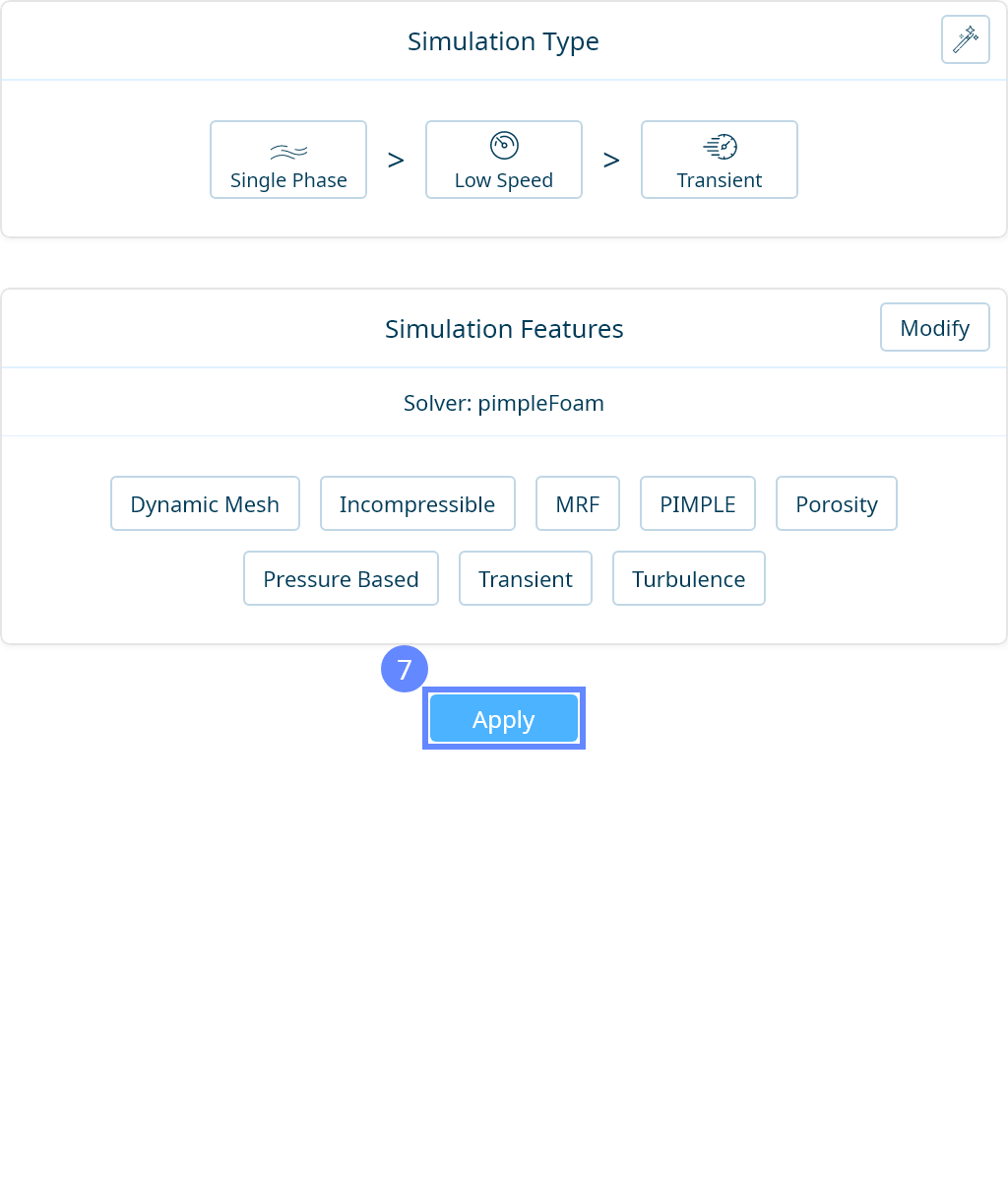
20. Simulation Type
We want to analyze the transient and incompressible flow in a static mixer. For this purpose, we will use a single-phase, transient, incompressible flow simulation.

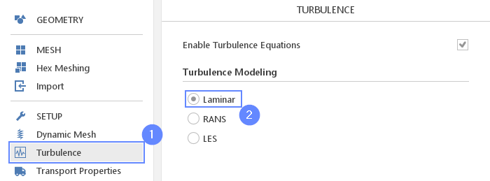
21. Turbulence
In this tutorial, we will consider a laminar flow.
- Go to Turbulence panel
- Make sure the Laminar model is selected
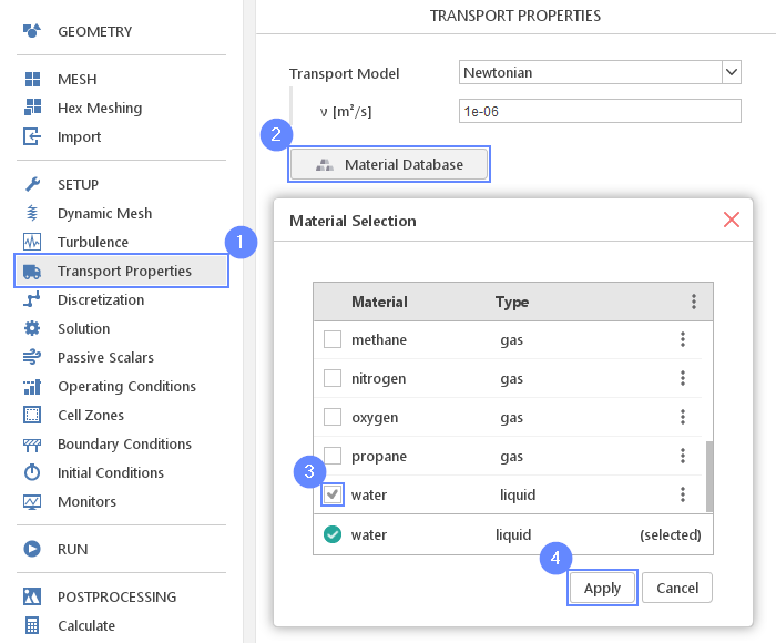
22. Transport Properties
In order to define water properties, we go to the transport properties panel. We will use predefined fluid properties from the material database.
- Go to Transport Properties panel
- Click on Material Database
- Select the water
- Click Apply
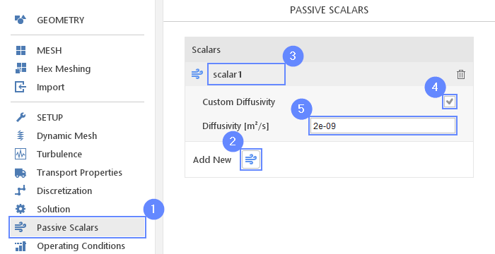
23. Passive Scalar
We will use passive scalar to simulate the mixing of two different fluids. Passive scalar adds an additional transport equation to the system of governing equations. Note, the passive scalar does not influence the flow itself but only introduces a marker for tracing fluid transport. The scalar takes a value between 0 and 1 (0 represents clear water, and 1 represents water with air dissolved in it). To control scalar properties we can define either the Schmidt number or custom diffusivity. In our case, we will define custom diffusivity equal 2.0e-09 which corresponds to the water-air mixture.
- Go to Passive Scalars panel
- Press Add new passive scalar Equations button
- Click on scalar1 to expand options list
- Check the Custom Diffusivity
- Set the diffusivity
Diffusivity \({\sf [m^2/s]}\)2e-09
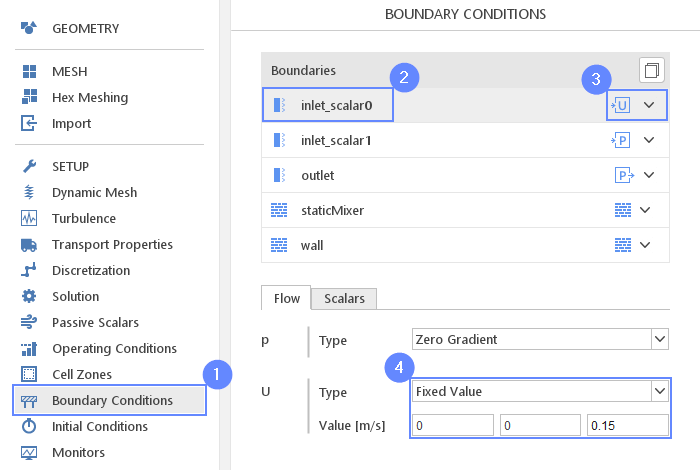
24. Boundary Conditions - Inlet Scalar 0 (Flow)
We will define the constant inlet velocity for both inlets.
- Go to Boundary Conditions panel
- Select inlet_scalar0 boundary
- Set the boundary character
inlet_scalar0 Velocity Inlet - Change the type and value of the velocity
UTypeFixed Value
UValue \({\sf [m/s]}\)000.15
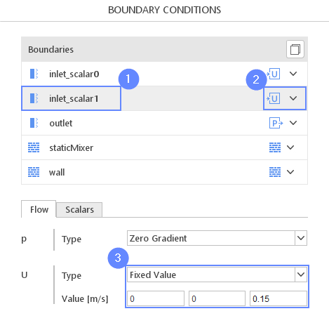
25. Boundary Conditions - Inlet Scalar 1 (Flow)
Repeat these steps for the second inlet.
- Select inlet_scalar1 boundary
- Set the boundary character
inlet_scalar1 Velocity Inlet - Change the type and value of the velocity
UTypeFixed Value
UValue \({\sf [m/s]}\)000.15
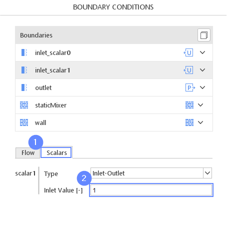
26. Boundary Conditions - Inlet Scalar 1 (Scalars)
For the inlet_scalar1 boundary set the inflow phase value.
- Switch to Scalars tab
- Set the value of scalar1 to:
scalar1Inlet Value \({\sf [-]}\)1
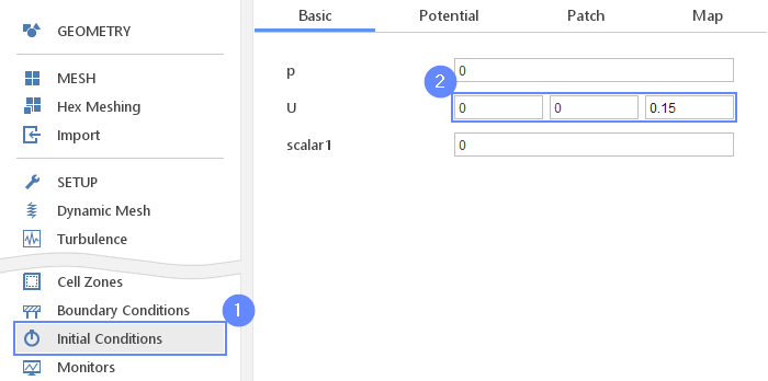
27. Initial Conditions
Before we start simulation we need to define the initial conditions. We will specify a constant velocity equal to 0.15 m/s which corresponds to the inlet velocity.
- Go to Initial Conditions panel
- Set the velocity
U 000.15
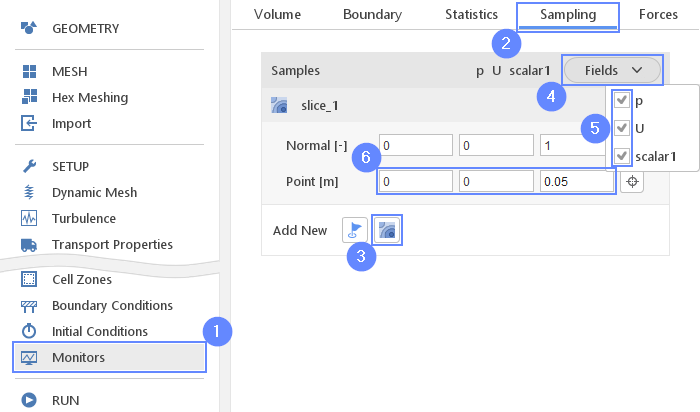
28. Monitors - Create Slice (I)
During calculation, we can observe intermediate results on a section plane. To add sampling data on a plane we need to define plane properties and also select variables that will be sampled. Note that runtime post-processing can only be defined before starting calculations and can not be changed later on.
- Go to Monitors panel
- Switch to Sampling tab
- Select Create Slice
- Expand Fields list
- Select all available options
Fields p U scalar1 - Normal is defined along Z axis. Set the point to:
Point \({\sf [m]}\)000.05
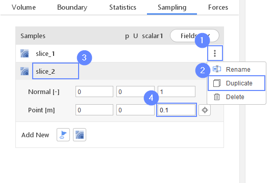
29. Monitors - Create Slice (II)
Create the next slice above the mixer.
- Expand Options list next to the slice_1
- Click Duplicate
- Click on slice_2 to expand options list
- Change the point coordinate
Point [m] 000.1
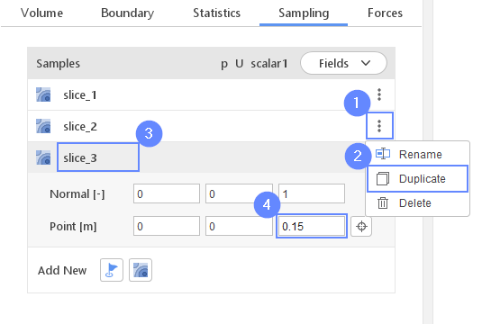
30. Monitors - Create Slice (III)
Duplicate the slice once again and move it to the vicinity of the outlet.
- Expand Options list next to the slice_2
- Click Duplicate
- Click on slice_3 to expand options list
- Change the point coordinate
Point [m] 000.15
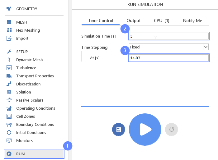
31. Run - Time Controls
Before running computations adjust the time controls in order to capture appropriate time scales of the flow features.
- Go to RUN panel
- Set the simulation time
Simulation Time [s] 3 - Set the time stepping
Time Stepping \(\Delta t[s]\) 1e-03
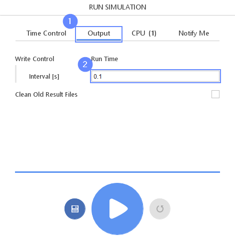
32. Run - Output
We can control how often results should be saved on the hard drive. We will write the results at the interval of ` 0.1 ` seconds. Note, that only saved data will be available during postprocessing.
- Switch to Output tab
- Set the write control interval
Write Control Interval [s] 0.1
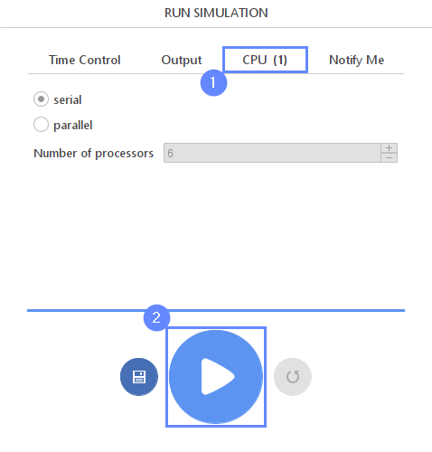
33. Run - CPU
To speed up the calculation process, take advantage of parallel computing and increase the number of CPUs based on your PC’s capability. The free version allows you to use only one processor (serial mode). To get the full version, you can use the contact form to Request 30-day Trial
Estimated computation time for serial mode: 30 minutes
- Switch to CPU tab
- Click Run Simulation button
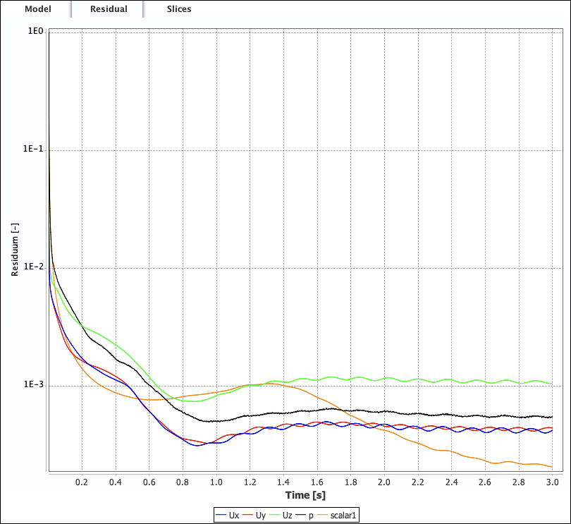
34. Residuals
When the calculation is finished, we should see a similar residual plot.
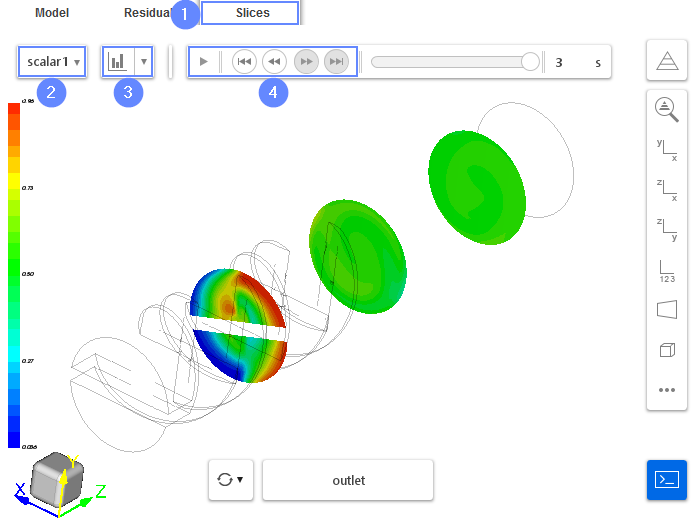
35. Results - Slice
Slices tab appears next to Residuals. Under this tab, we can preview results on the defined slice planes. The results preview is available during the calculation and we can track it on a regular basis. The newly calculated time step will be actualized automatically as long as the time selector points to the latest time step.
We want to check if the fluids are mixed at the end of the mixer. We will display scalar1 contribution at each slice in the mixer.
- Change tab to Slice
- Changed displayed results by selecting scalar1
- To adjust color range to actually displayed data click Adjust range to data
- Play with animation buttons to view the results of the analysis.
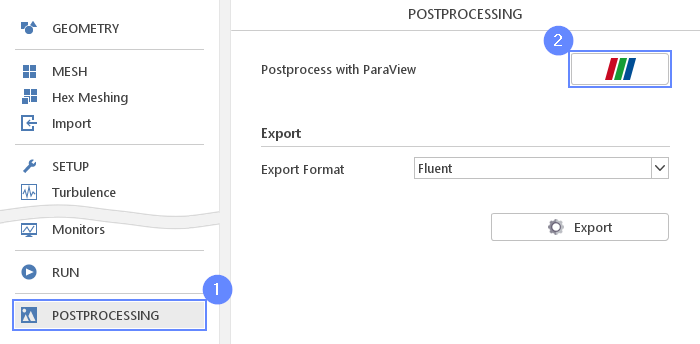
36. Postprocessing - ParaView
After computations are finished we can do complex visualization of our results with ParaView.
- Go to POSTPROCESSING panel
- Click on Run ParaView
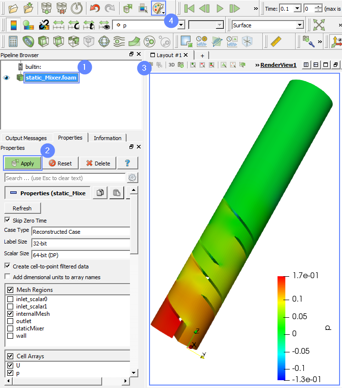
37. ParaView - Load Results
Load the results into the program.
- Select static_mixer.foam
- Click Apply to load results into ParaView
- After loading results they will be shown in the 3D graphic window
- Click on a Load a colour palette from the top menu and select White Background
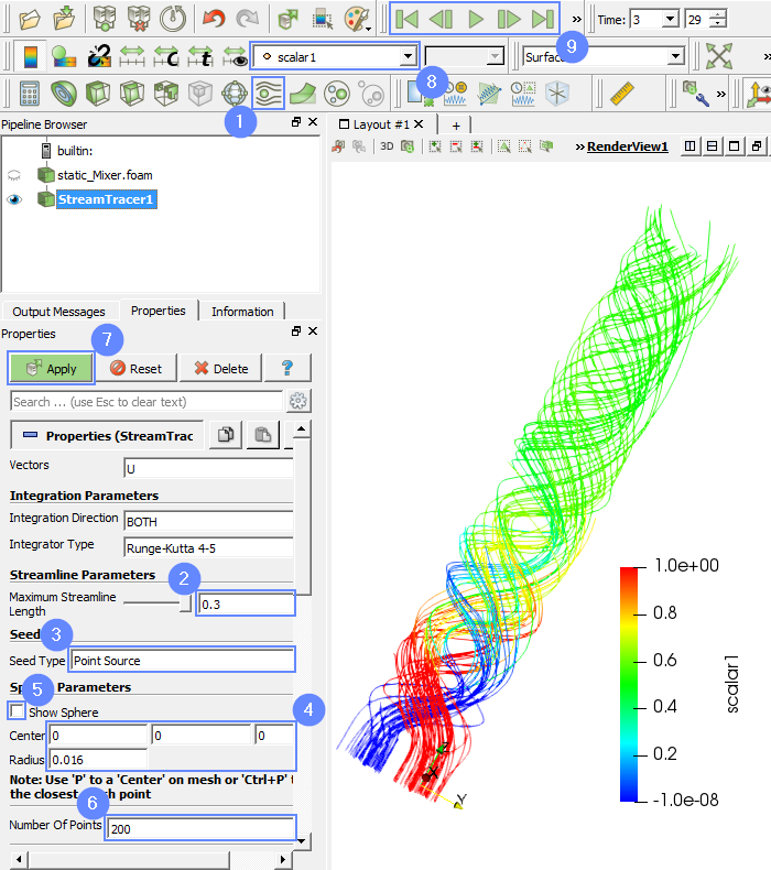
38. ParaView - Streamline (I)
We can visualize the flow by displaying the streamlines.
- Select Stream Tracer from top menu
- Set the maximum streamline length
Maximum Streamline Length 0.3 - Change a seed type
Seed Type Point Source - Type the center coordinate and radius of the sphere:
Center000
Radius0.016 - Uncheck the Show Sphere
- Increase the number of points
Number of Points 200 - Click Apply
- Select the scalar1 from the list
- Play with animation buttons to track the results of the analysis.
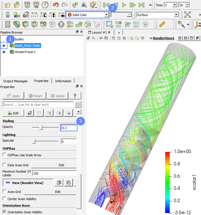
39. ParaView - Streamline (II)
To show the geometry together with the streamlines we will follow below steps:
- Click on the eye next to static_mixer.foam
- Select Solid Color from the list
- Change the opacity
Opacity 0.3