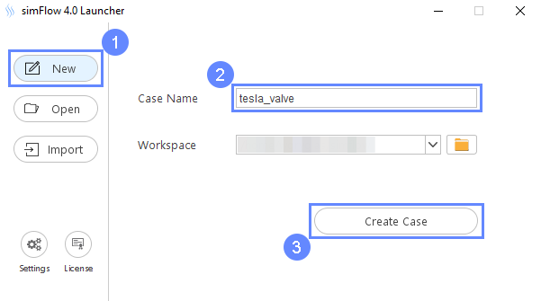
3. Create Case
Open SimFlow and create a new case named tesla_valve
- Go to New panel
- Provide name tesla_valve
- Click Create Case
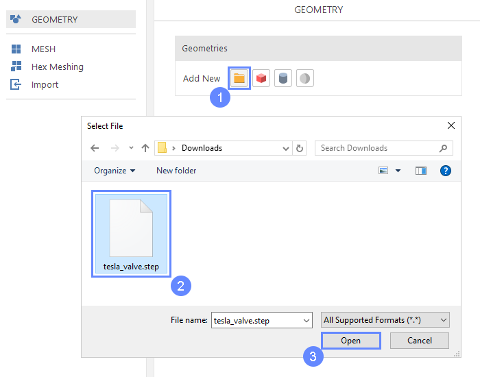
4. Import Geometry - Tesla Valve
Firstly we need to Download GeometryTesla_valve. The geometry will be imported in the same units as it was exported to the STEP format.
- Click Import Geometry
- Select geometry file tesla_valve.step
- Click Open
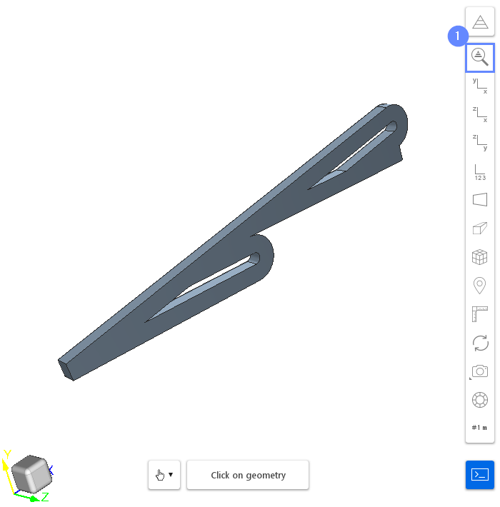
5. Geometry - Tesla Valve
After importing geometry, it will appear in the 3D window.
- Click Fit View to fit geometry in the view

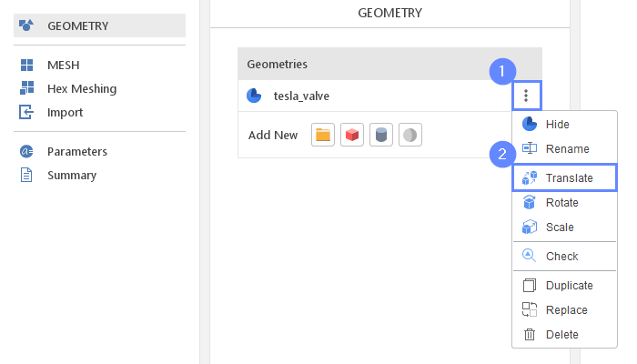
6. Translate Geometry - Tesla Valve (I)
The geometry is a three-dimensional volume. However, in this tutorial, we will work on a two-dimensional case. To prepare this kind of mesh, we will use the Plate (2D plane) base mesh, which should cut through the 3D volume. Therefore, we need to adjust the location of the geometry so that its center will be located on the XY plane.
- Expand the Options list for tesla valve
(you can also right-click on geometry name) - Select Translate
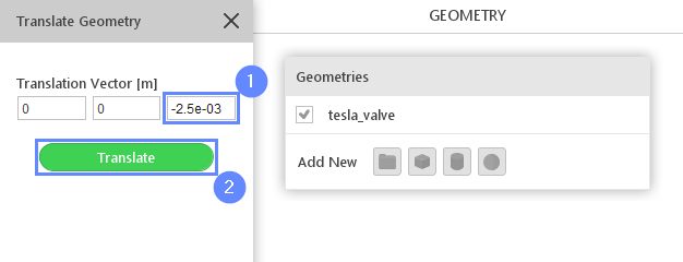
7. Translate Geometry - Tesla Valve (II)
Now we have to specify coordinates for the translation.
- Set translation vector
Translation Vector \({\sf [m]}\)00-2.5e-03 - Click Translate
8. Preview Geometry
After the geometry is scaled we will not be able to see it in the 3D graphics panel. We can adjust the view by using the Fit View button.
- Select Fit View
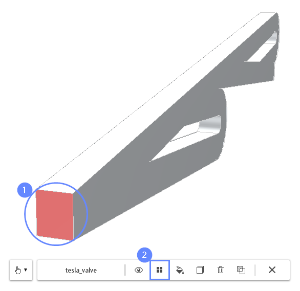
9. Creating Face Groups (I)
In this fluid flow simulation, we are dealing with an internal flow problem. The imported geometry determines the bounds of the fluid domain. To inform the program where the boundaries of the inlet and outlet mesh should be created, we will use the Face Groups options. Face Groups can be created directly in the 3D graphics panel or from the Face Group geometry properties panel. In this tutorial, we will utilize the first approach.
- Select the inlet face by holding CTRL button and clicking on the geometry face in a 3D view. The selection should be marked in red
- Click on the Face Group button in the graphics context toolbar
- Press Esc key to clear the selection
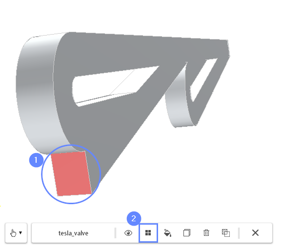
10. Creating Face Groups (II)
Next, rotate the view in such a way that you will be able to see the second end of the geometry.
- Select the outlet face by holding CTRL button and clicking on the geometry face
- Click on the Face Group button in the graphics context toolbar
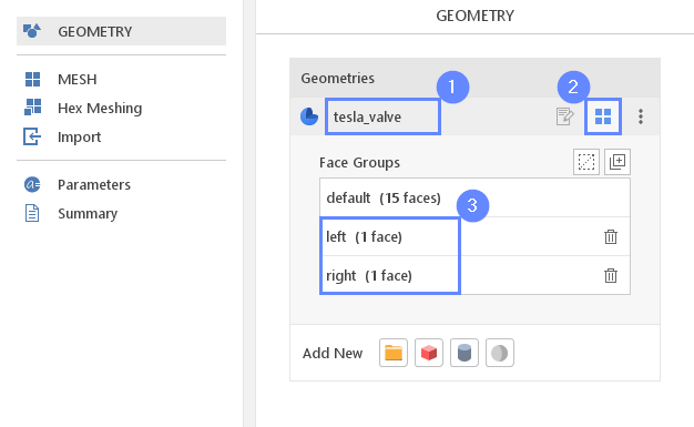
11. Rename Face Groups
In the Geometry Panel we can find three Face Groups under the tesla_valve geometry. The first group, named default, contains all non-selected surfaces. These surfaces will constitute the walls of the valve. The two additional groups represent the inlet and outlet of the fluid domain. We will rename those groups to make the resulting boundary names more readable.
- Select tesla_valve geometry
- Expand Geometry Faces
- Change face groups names accordingly
group_1 \(\rightarrow\) left
group_2 \(\rightarrow\) right
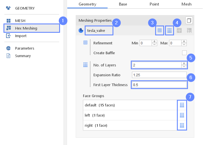
12. Meshing Parameters - Tesla Valve
In order to create the mesh, we need to specify geometries features used during the meshing process.
- Go to Hex Meshing panel
- Select the tesla_valve component
- Enable Mesh Geometry
- Enable Create Boundary Layer Mesh
- Set No. of Layers to 2
- Set First Layer Thickness to 0.5
(by default first cell size value is the relative size, in this case, the program will generate a boundary layer with a height equal to half of the original near wall cell) - Select all Face Groups for Boundary Layer Mesh
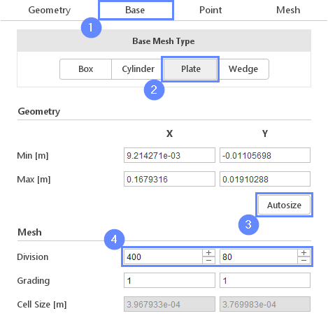
13. Base Mesh - Domain
We are going to create a mesh for a 2D fluid flow problem. The Plate base mesh is best suited for this purpose. This base mesh type will automatically take care of preparing appropriate boundaries for Z-direction.
- Go to Base tab
- Select the Plate as a Base Mesh Type
- Click on Autosize
- Define the number of divisions
Division40080
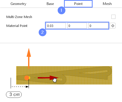
14. Material Point
Material Point tells the meshing algorithm on which side of the geometry the mesh is to be retained. Since we are considering flow inside the mold we need to place the material point inside the geometry.
- Go to Point tab
- Specify location inside tesla_valve geometry
Material Point0.0300
You can specify the point location from the 3D view. Hold the CTRL key and drag the arrows to the destination.
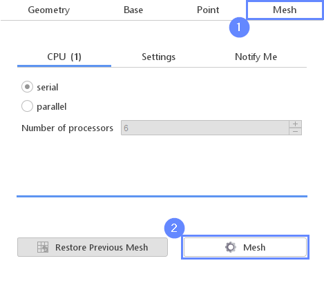
15. Start Meshing
Everything is now set up for meshing.
- Switch to Mesh tab
- Start the meshing process with Mesh button
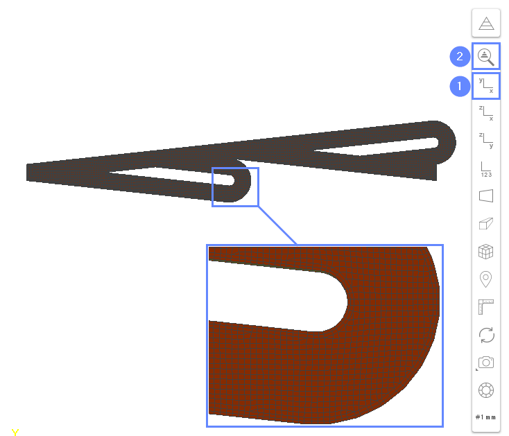
16. Check Mesh
After the meshing process is finished the mesh should appear in the graphics window.
- Set the XY orientation View XZ
- Click Fit View
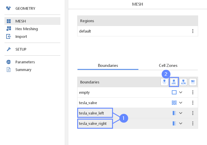
18. Boundary Coupling (II)
Now we will create AMI coupling between the left and the right side of the valve segment.
- Hold CTRL key and select both tesla_valve_left and tesla_valve_right boundaries
- Click the Cyclic AMI
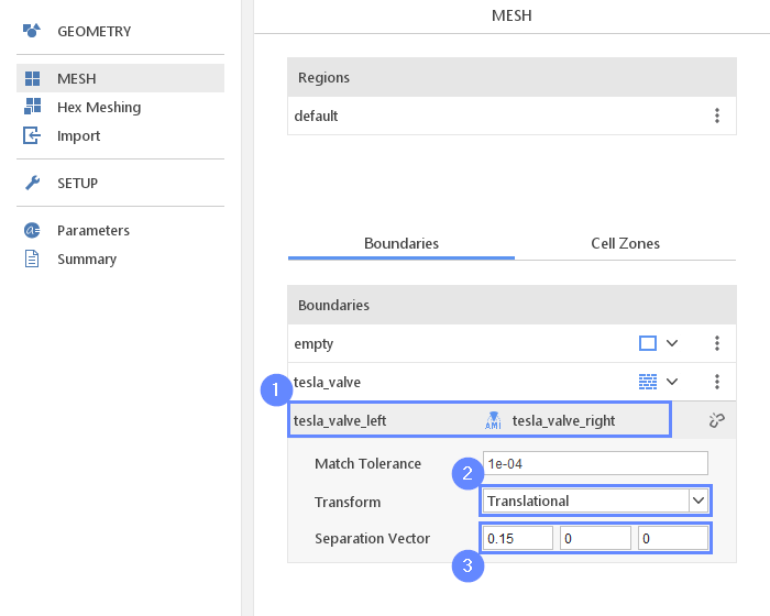
19. AMI Properties
- Click on coupled boundary to display properties
- Select Translational transform
- Set the vector between left and right boundary
Separation Vector0.1500
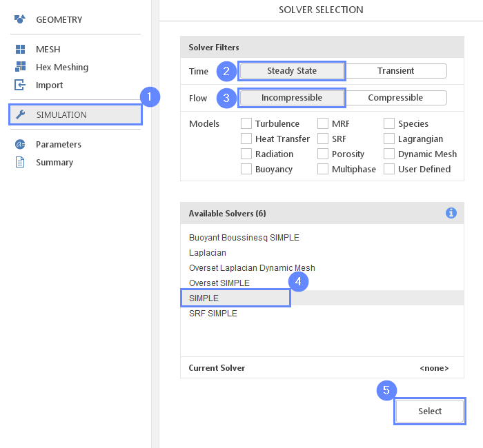
20. Select Solver - SIMPLE
We want to analyze incompressible turbulent flow inside the tesla valve. For this purpose, we will use the SIMPLE (simpleFoam) solver.
- Go to SETUP panel
- Select Steady State type
- Select Incompressible flow filter
- Select SIMPLE (simpleFoam) solver
- Select solver
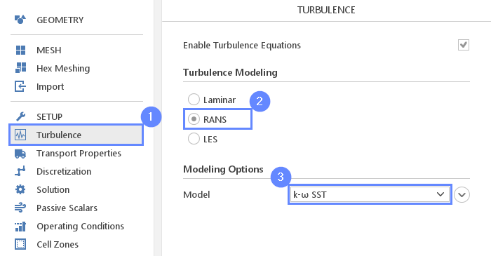
21. Turbulence
We are going to use the standard \(k{-}\omega \; SST\) model to handle turbulence.
- Go to Turbulence panel
- Select RANS modeling
- Select \(k{-}\omega \; SST\) model
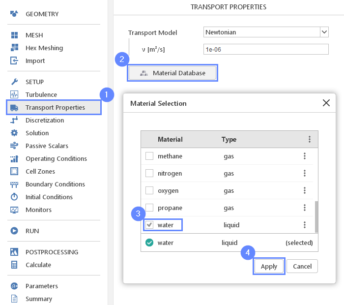
22. Transport Properties - Water
As a fluid material, we will use water.
- Go to Transport Properties panel
- Open Material Database
- Pick up water from the list
- Click Apply
Selecting material from the Material Database will fill all inputs in the Transport Properties panel. At any time we will still be able to overwrite these values.
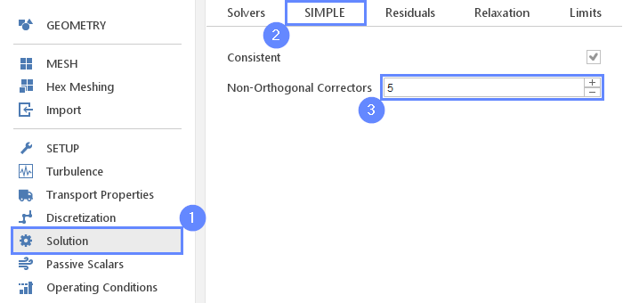
23. Solution - SIMPLE
We will also modify the solver configuration what will increase the stability of the computational process.
- Go to Solution panel
- Switch to the SIMPLE tab
- Increase the Non-Orthogonal Correctors to 5
This option usually improves stability and convergence but at an additional computational cost due to solving pressure equations multiple times.
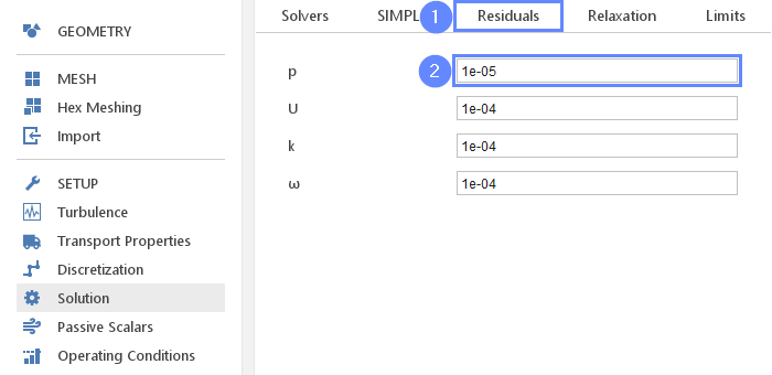
24. Solution - Residuals
We will decrease residual levels for pressure. We do not need to decrease the residual level for other variables because the pressure equation is usually the one converging last.
- Switch to the Residuals tab
- Change the pressure residual to
p1e-05
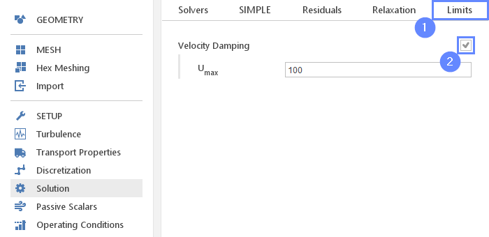
25. Solution - Limits
Velocity Dumping can prevent the solver from diverging even if nonphysical velocity would appear during the iterations.
- Switch to the Limits tab
- Check the Velocity Damping
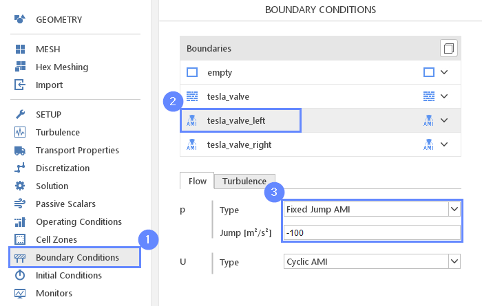
26. Boundary Conditions
We are simulating one segment of a periodic geometry, where values at the inlet and outlet of the domain are bounded by the cyclic constraint. In this case, we can not force fluid flow by using a standard approach, but we will use pressure jump instead. This boundary condition will force constant pressure difference between coupled boundaries.
- Go to Boundary Conditions panel
- Select tesla_valve_left boundary
- Set the pressure type and jump value accordingly
p TypeFixed Jump AMI
p Jump \({\sf [m^2 / s^2]}\)-100
If, after changing boundary condition type to Fixed Jump AMI you do not see the Jump input field then move to the tesla_valve_right boundary, where this input will appear. In this case, you will have to apply the pressure difference with an opposite sign. The Jump value input appears only on master boundary, which is the first boundary in the coupling.
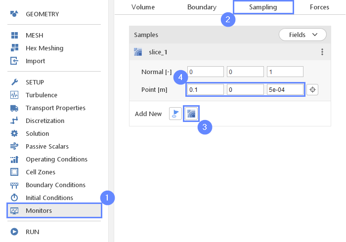
27. Monitors - Sampling (I)
During calculation, we can observe intermediate results on a section plane. To add sampling data on a plane we need to define plane properties and also select fields that will be sampled. Note that runtime post-processing can only be defined before starting calculations and can not be changed later on.
- Go to Monitors panel
- Switch to Sampling tab
- Select Create Slice
- Set slice plane location
Point \({\sf [m]}\)0.105e-04
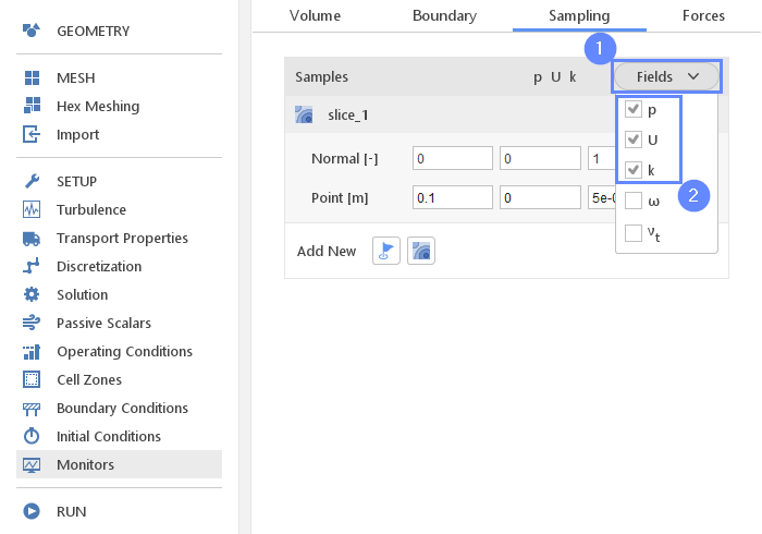
28. Monitors - Sampling (II)
Additionally, to specifying section plane geometry we need to choose which results should be sampled on the surface.
- Expand Fields list
- Select pressure p , velocity U and turbulence kinetic energy k
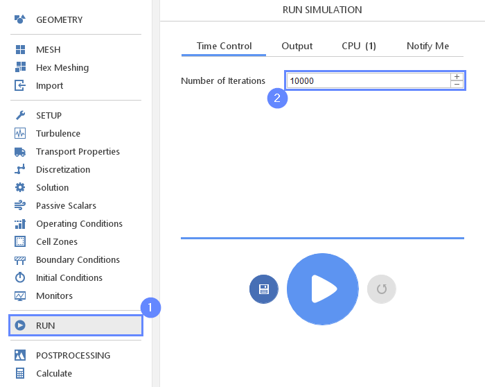
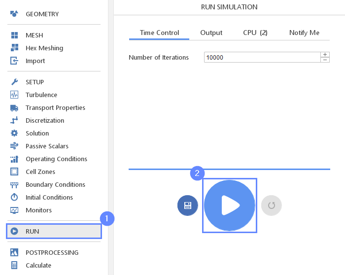
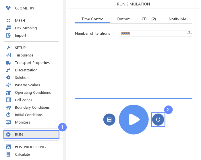
29. Run - Time Control
Finally, we can start our computation.
- Go to RUN panel
- Set the maximum Number of Iteration to 10000
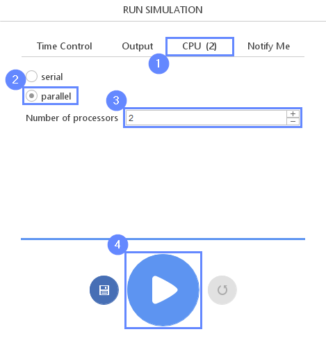
30. Run - CPU
To speed up the calculation process increase the number of CPUs basing on your PC capability. The free version allows you to use only 2 processors in parallel mode. To get the full version, you can use the contact form to Request 30-day Trial
Estimated computation time for 2 processors: 3 minutes
- Switch to CPU tab
- Use parallel mode
- Increase the Number of processors
- Click Run Simulation button
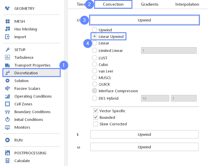
31. Discretization - Convection
After preliminary calculation, we will continue with a more accurate algorithm. Change velocity discretization to the Linear Upwind scheme to minimize numerical diffusion affecting the results of the simulation.
- Go to the Discretization panel
- Switch to Convection tab
- Click on Upwind to extend the list
- Change scheme to Linear Upwind
32. Run - Continue Simulation
Move back to Run panel and continue calculation. Note we did not remove the previous result but we use them as a starting point for computation with a higher-order scheme.
- Go to RUN panel
- Click Continue Simulation button
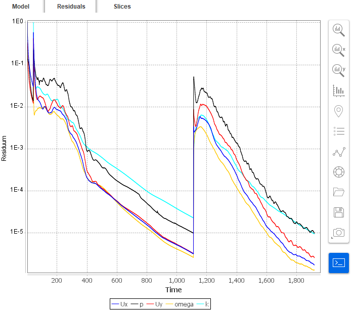
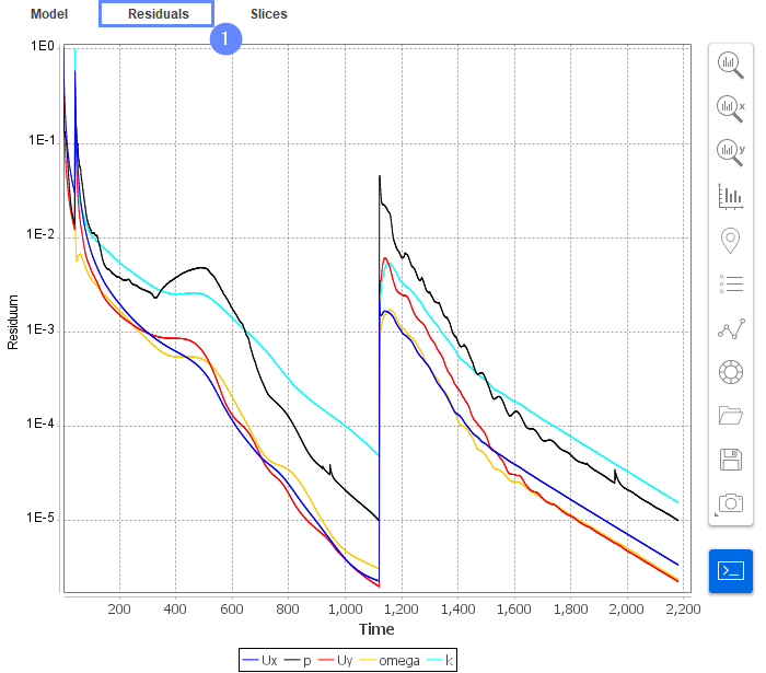
33. Residuals
When the calculation is finished we should see a similar residual plot. Note that we can see how residual values get up when we have changed the convection scheme. This is due to the fact that different numerical scheme results in slightly different discrete equations which do not match results from previous calculations.
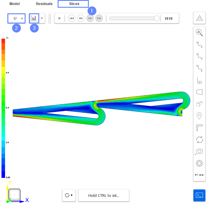
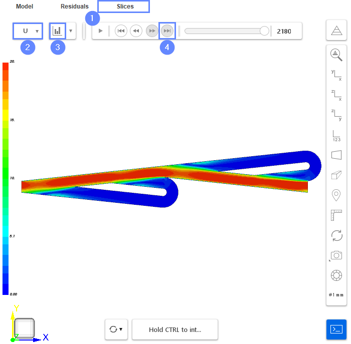
34. Slice - Velocity Field
Slices tab appears next to the Residuals tab. Under this tab, we can preview results on the defined section plane.
- Change tab to Slices
- Select the velocity U
- Click Adjust range to data
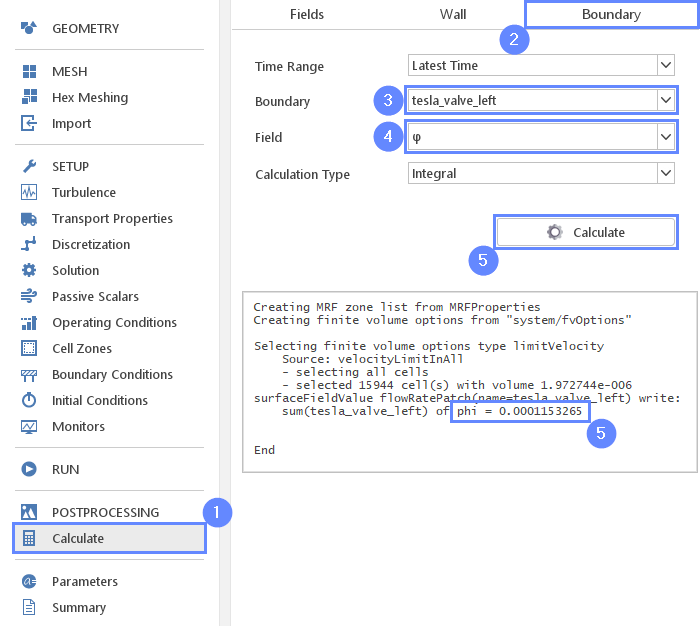
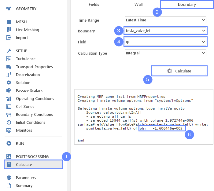
35. Calculate - Mass Flow Rate
Finally, we will calculate what is the mass flow rate in the flow blocking direction.
- Go to Calculate panel
- Switch to Boundary tab
- Select tesla_valve_left boundary
- Choose the \(\varphi\) variable
- Click the Calculate button
- Read the phi value from the console
Results will be displayed in the console. The \(\phi\)φ variable is the flux through mesh faces. In the case of incompressible solvers, the flux is volumetric instead of mass flux. To obtain mass flow rate we have to multiply results by reference density.
36. Reset Result
In the next simulation, we will invert flow direction and once again compute the flow rate forced by the same pressure gradient.
- Go back to RUN panel
- Click Reset Calculation button. This will remove current results and allow to change setting for the second simulation
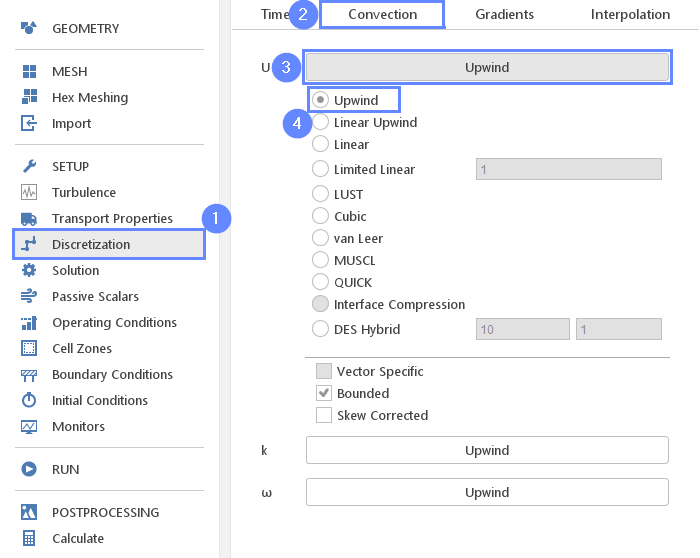
37. Reset Discretization Setup
We need to change the higher-order Linear Upwind scheme back to Upwind . This scheme will be again used for initial calculation since it is less accurate but more stable.
- Go to Discretization panel
- Switch to Convection tab
- Expand the scheme list for U
- Change scheme to Upwind
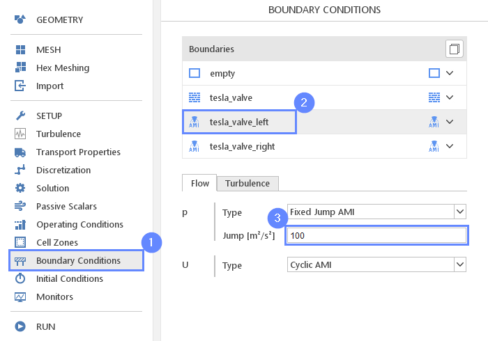
38. Boundary Conditions -Inverse Pressure Gradient
In the second run, we will investigate the results with fluid moving in the opposite direction.
- Go to Boundary Conditions panel
- Select the tesla_valve_left boundary
- Set the Jump value to 100
39. Run - Second Simulation
We leave the rest of the configuration unchanged. Now we can start the new calculation.
- Go to RUN panel
- Click Run Simulation button

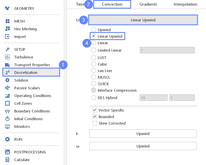
40. Discretization - Convection (2nd Case)
Again, after preliminary calculation, we will continue with a more accurate algorithm.
- Go to Discretization panel
- Switch to Convection tab
- Expand the scheme list for U
- Change scheme to Linear Upwind
41. Run - Continue Calculation (2nd Case)
Move back to Run panel and continue calculation.
- Go to RUN panel
- Click Continue Simulation button

42. Residuals (2nd Case)
When the calculation is finished we should see a similar residual plot.
- Switch to Residuals tab
43. Slice - Velocity Field (2nd Case)
As previously change tab to Slices and display velocity field. Compare results with previous velocity field. We can see that the velocity level is much higher under the same pressure gradient, which indicates that this configuration results in much smaller resistance.
- Change tab to Slices
- Select the velocity U
- Click Adjust range to data
- Display the latest results by clicking End button
44. Calculate - Mass Flow Rate (2nd Case)
Finally, we will calculate the mass flow rate for the second simulation and compare the results.
- Go to Calculate panel
- Switch to Boundary tab
- Select tesla_valve_left boundary
- Choose the \(\varphi\) variable
- Click the Calculate button
- Read the phi value from the console
The sign of mass flow rate defines the direction of the flow. This time the value is positive because fluid flows outside the domain. We are interested only in absolute values. Check the ratio of mass flow rates between the two simulations:
\(Ratio = \frac{0.000115}{1.606e-005} \approx 7.2\)
As we can see, the 7.2 times more fluid flowing through the valve when we apply a pressure difference in the forward direction. Note that this simulation is in 2D, which means that the valve is infinitely wide and does not account the resistance from the side walls.