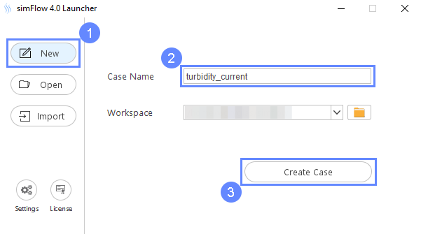
3. Create Case
Open SimFlow and create a new case named turbidity_current
- Go to New panel
- Provide name turbidity_current
- Click Create Case
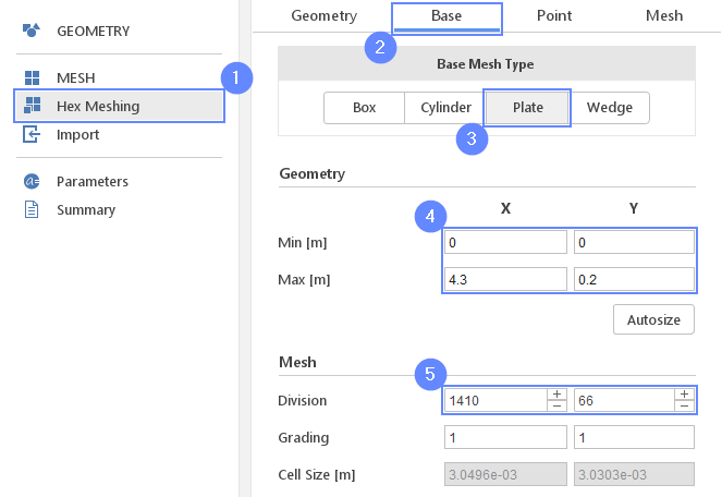
4. Base Mesh
In this tutorial, we consider a 2D simulation where the base mesh defines the entire tank. To do this we will use the Plate type which lets us create rectangular grid.
- Go to Hex Meshing panel
- Switch to Base tab
- Select the Plate as a Base Mesh Type
- Set the size of the base mesh
Min \({\sf [m]}\)00
Max \({\sf [m]}\)4.30.2 - Define the number of divisions
Division141066
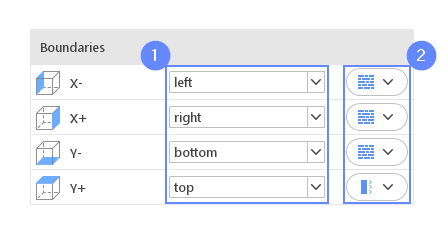
5. Base Mesh Boundaries
We need to assign individual names to each side of the base mesh. This will allow us to apply different conditions to each side.
- Define boundary names accordingly
X- left
X+ right
Y- bottom
Y+ top - Define boundary types accordingly
X- wall
X+ wall
Y- wall
Y+ patch
6. Start Meshing
Everything is now set up for meshing.
- Go to Mesh tab
- Press the Mesh button to start meshing process
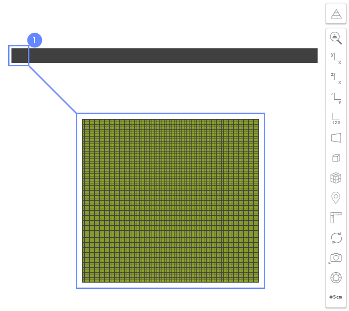
7. Mesh
After the meshing process is finished the mesh will appear in the graphics window.
- Zoom in to the left side of the mesh - use the Scroll Wheel or drag mouse with RMB (right mouse button) pressed
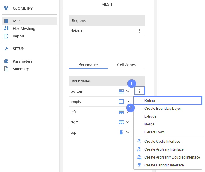
8. Refine Mesh - Bottom (I)
We will refine the mesh to improve spatial discretization in the near-wall region. It is important in the initial location of the fluid mud suspension. To increase near-wall mesh resolution we usually add a boundary layer during the meshing process. However, SimFlow allows modifying existing mesh as well. We can add a boundary layer to a selected boundary or we can split near-wall cells. The latter option is very handy when it is required to refine boundary layer cells in order to advise desired y+ value without remeshing whole domains. In this tutorial, we will demonstrate the usage of the splitting approach.
- Expand options list for bottom boundary
- Select Refine
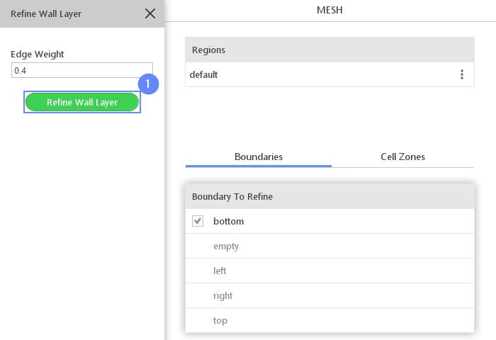
9. Refine Mesh - Bottom (II)
Refine Wall Layer option will divide the first cell adjacent to the boundary into two cells.
- Select Refine Wall Layer
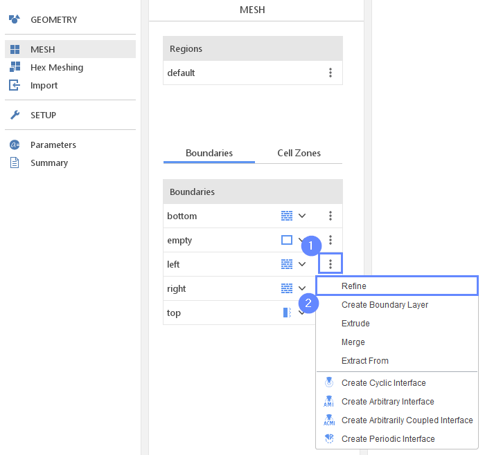
10. Refine Mesh - Left (I)
We will also refine the mesh for the left boundary in the same manner.
- Expand options list for left boundary
- Select Refine
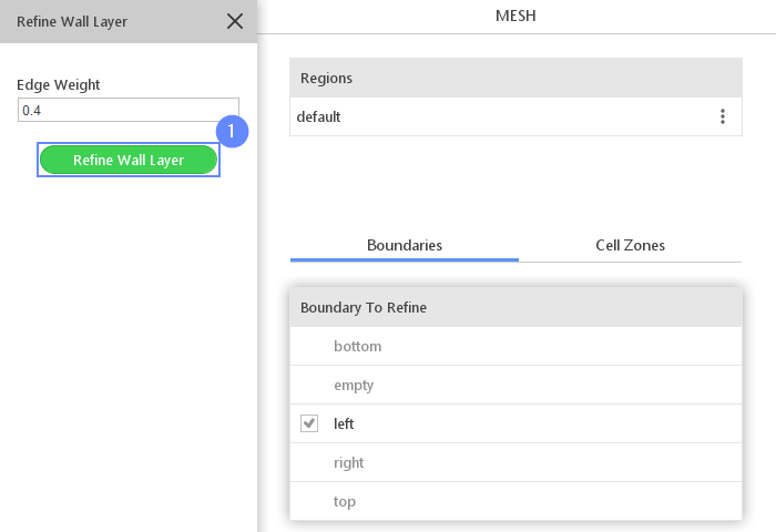
11. Refine Mesh - Left (II)
- Select Refine Wall Layer
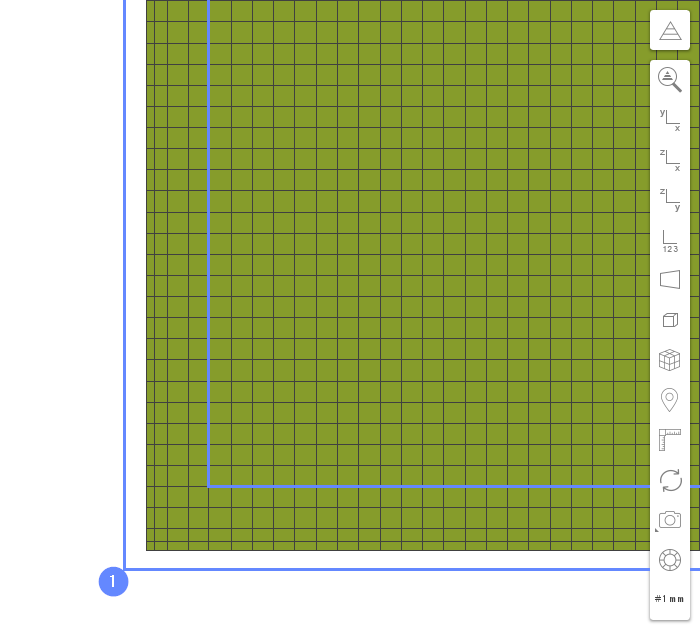
12. Examine Mesh
After the refining process is finished the mesh should appear in the graphics window. Use the scroll wheel in your mouse to zoom in the left bottom corner and examine the mesh refinement region.
- Zoom in to the bottom left corner of the mesh
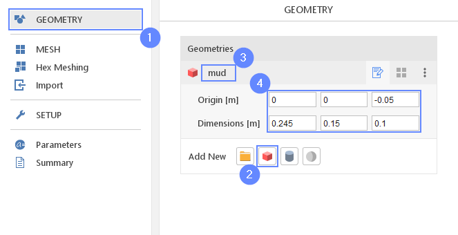
13. Create Geometry - Mud
The initial mesh represents the entire tank. We need to specify where the mud suspension and water are initially located inside the domain. For this purpose, we need to create additional geometries.
- Go to Geometry panel
- Select Create Box
- Change geometry name from box_1 to mud
(double click to edit name and press Enter to confirm) - Set the origin and box dimensions
Origin \({\sf [m]}\)00-0.05
Dimensions \({\sf [m]}\)0.2450.150.1
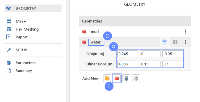
14. Create Geometry - Water
The second box defines the water phase.
- Select Create Box
- Change geometry name from box_1 to water
- Set the origin and box dimensions
Origin \({\sf [m]}\)0.2450-0.05
Dimensions \({\sf [m]}\)4.0550.150.1
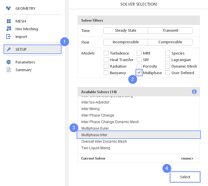
15. Select Solver - Multiphase Inter
We want to analyze transient, incompressible flow with several isothermal and immiscible fluids. For this purpose, we will use the Multiphase Inter (multiphaseInterFoam) solver.
- Go to SETUP panel
- Filter the solvers by choosing Multiphase models
- Pick Multiphase Inter (multiphaseInterFoam) solver
- Select solver
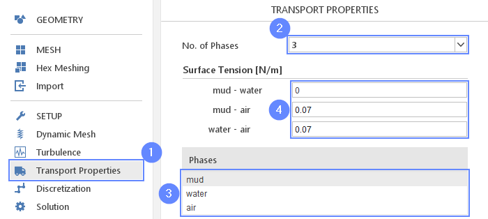
16. Transport Properties - Phases
We need to define the properties for three phases: mud, water and air. To assign material to the domain, the phase fraction parameter \(\alpha_{phase}\) is used. The parameter determines the proportion of each fluid in the domain. The value of phase fraction varies in range from 0 to 1 where \(\alpha_{phase1}=1\) means that the whole domain is filled only with the phase1, while \(\alpha_{phase1}=0\) means that the domain is filled with the second phase.
- Go to Transport Properties panel
- Set the No. of Phases to 3
- Rename the phases respectively
phase1 \(\rightarrow\) mud
phase2 \(\rightarrow\) water
phase3 \(\rightarrow\) air - Set the Surface Tension [N/m] for each pair as follows
mud - water0
mud - air0.07
water - air0.07
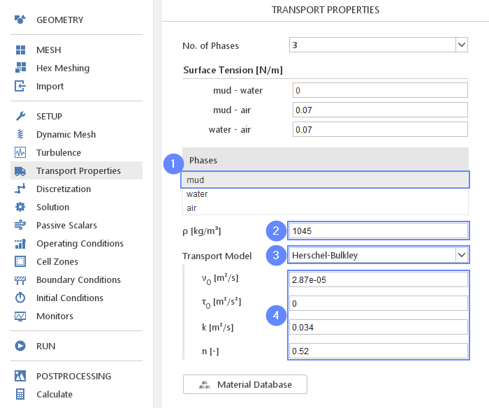
17. Transport Properties - Mud
- Select the mud from the Phases list
- Set the density \(\rho \; [kg/m^3] \) to 1045
- Change Transport Model to Herschel-Bulkley
- Set the parameters accordingly
\(\nu_0\) \({\sf [m^2/s]}\)2.87e-05
\(\tau_0\) \({\sf [m^2 / s^2]}\)0
\(k\) \({\sf [m^2/s]}\)0.034
\(n\) \({\sf [-]}\)0.52
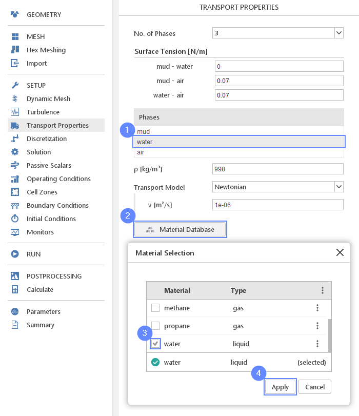
18. Transport Properties - Water
- Select the water from the Phases list
- Click Material Database
- Select the water
- Click Apply
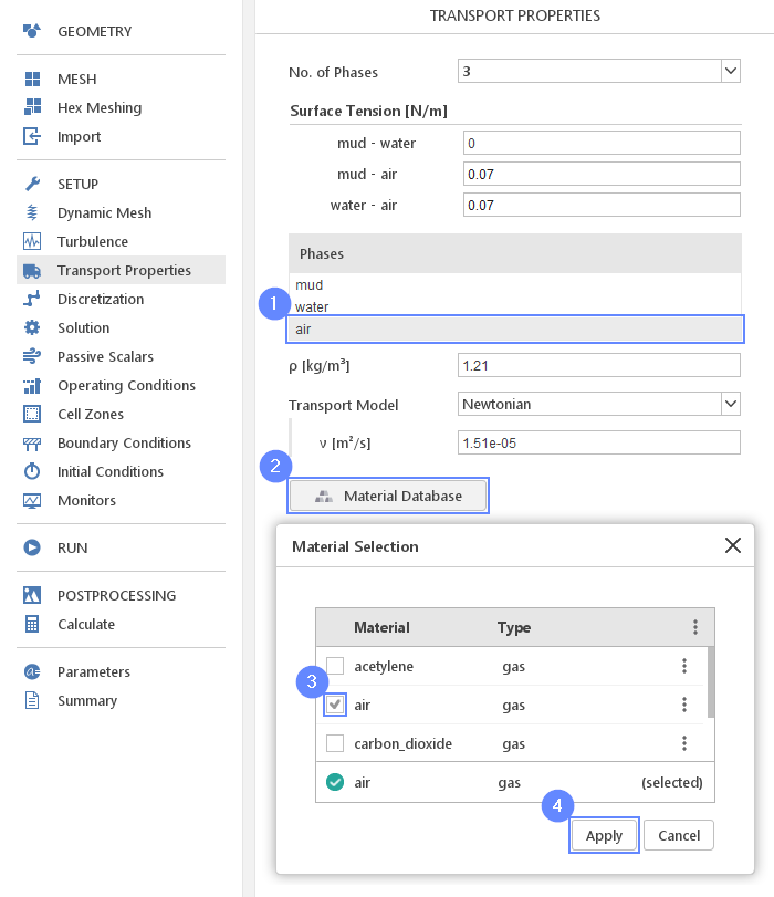
19. Transport Properties - Air
- Select the air from the Phases list
- Click Material Database
- Select the air
- Click Apply
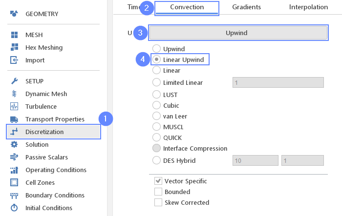
20. Discretization - Convection
Change the velocity discretization to the Linear Upwind scheme to minimize numerical diffusion affecting the results of the simulation.
- Go to Discretization panel
- Switch to Convection tab
- Click on default scheme Upwind
- Select Linear Upwind
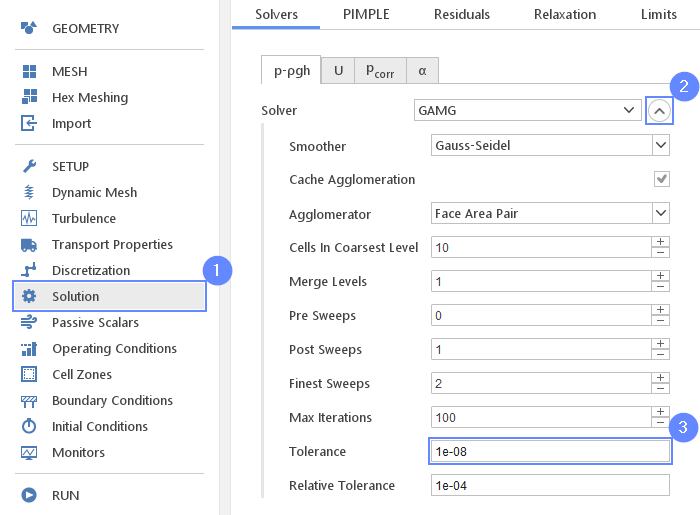
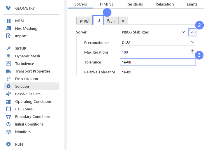
21. Solution - Tolerance (I)
To improve the simulation accuracy and stability for linear solver we will lower the tolerance used for pressure and velocity and increase the number of correction loops.
- Go to Solution panel
- Expand solver parameters
- Change Tolerance to 1e-08
22. Solution - Tolerance (II)
Similarly, for the velocity field.
- Switch to U tab
- Expand solver parameters
- Change Tolerance to 1e-08
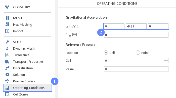
23. Operating Conditions - Gravity
Now we will set the appropriate vector of gravitational acceleration pointing in the negative direction of the y-axis.
- Go to Operating Conditions panel
- Define gravitational acceleration along negative Y axis
g \({\sf [m/s^2]}\)0-9.810
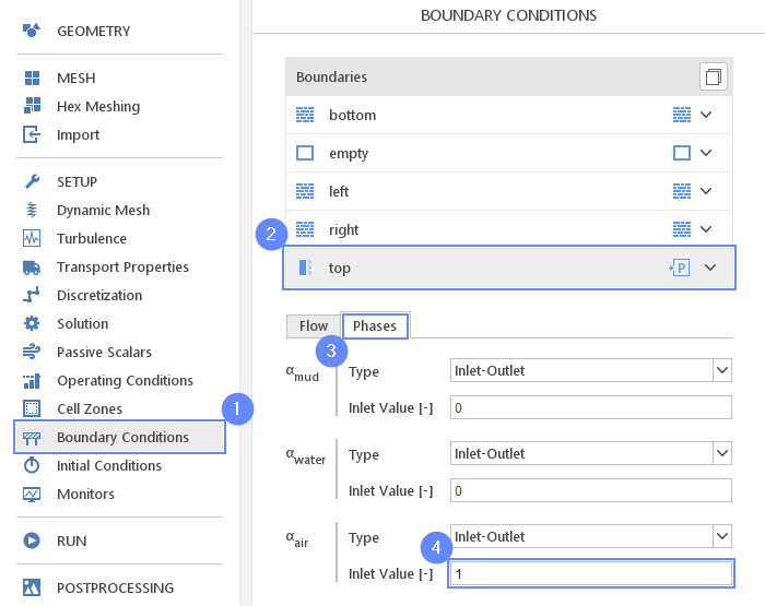
24. Boundary Conditions - Top
We will specify that air is the only phase flowing in or out of the domain across the top boundary.
- Go to Boundary Conditions panel
- Select top boundary
- Switch to Phases tab
- Set mass fraction of air
\(\alpha_{air}\) Inlet Value \({\sf [-]}\)1
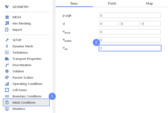
25. Initial Conditions - Basic
Before we start simulation we need to define the initial state. Phase fraction \(\alpha_{air}\) tells us that the whole domain is filled with the air by default.
- Go to Initial Conditions panel
- Set air phase fraction \(\alpha_{air}\) to 1
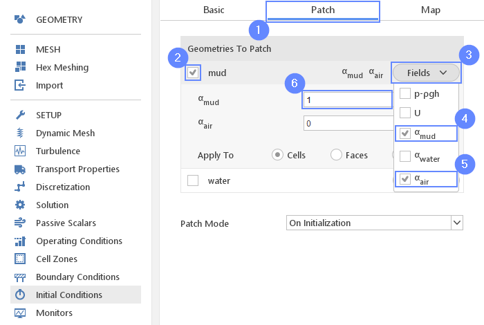
26. Initial Conditions - Patch Mud
Using the mud geometry, we will overwrite the phase fraction value inside it. We will set the \(\alpha_{mud}\) to 1 to fill the patched geometry with the mud suspension.
- Switch to Patch panel
- Enable initialization on mud geometry
- Expand the Fields list
- Select \(\alpha_{mud}\) fraction for initialization
- Select \(\alpha_{air}\) fraction for initialization
- Patch the form \(\alpha_{mud}\) with the value of 1
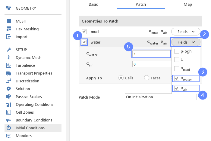
27. Initial Conditions - Patch Water
Similarly, using the water geometry, we will overwrite the phase fraction value inside it. We will set the \(\alpha_{water}\) to 1 to fill the patched geometry with the water.
- Enable initialization on water geometry
- Expand the Fields list
- Select \(\alpha_{water}\) fraction for initialization
- Select \(\alpha_{air}\) fraction for initialization
- Patch the form \(\alpha_{water}\) with the value of 1
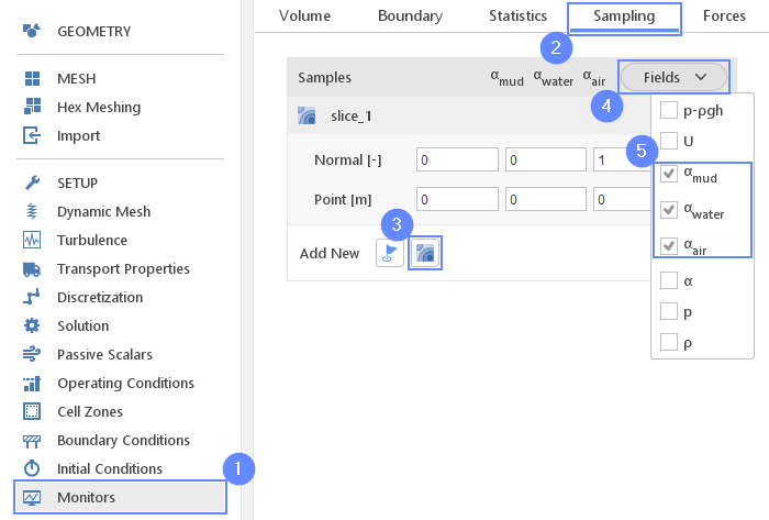
28. Monitors - Create Slice
During calculation, we can observe intermediate results on a section plane. To add sampling data on a plane we need to define plane properties and also select fields that will be sampled. Note that runtime post-processing can only be defined before starting calculations and can not be changed later on.
- Go to Monitors panel
- Switch to Sampling tab
- Add new Slice
- Expand Fields menu.
- Choose \(\alpha_{mud}\), \(\alpha_{water}\), \(\alpha_{air}\) to be sampled on the section plane.
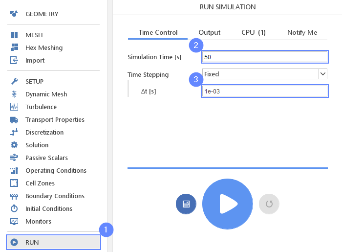
29. Run - Time Control
Before running computations adjust the time controls in order to capture appropriate time scales of the flow features.
- Go to RUN panel
- Set the Simulation Time [s] to 50
- Set the Time Stepping \(\Delta t\) [s] to 1e-03
This calculation will require high CPU usage and might take several hours to finish the calculation depending on the machine used. If you want to shorten the computation time, you can decrease the Simulation Time to 10s - this is enough for purpose of further postprocessing.
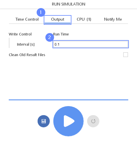
30. Run - Output
We can control how often results should be saved on the hard drive. Only this data will be available for postprocessing. We will write the results in the interval of 0.1 seconds.
- Switch to Output tab
- Set the Interval [s] to 0.1
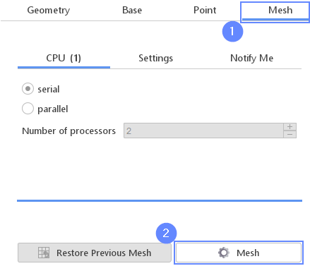
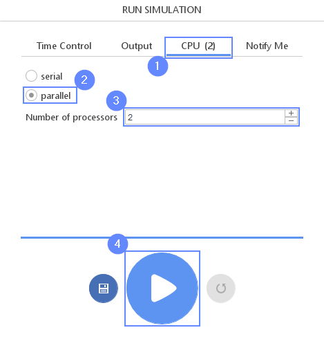
31. Run - CPU
To boost the calculation we can use a higher number of CPUs. We recommend using at least 8 processors for this tutorial. The free version allows you to use only 2 processors in parallel mode. To get the full version, you can use the contact form to Request 30-day Trial
Estimated computation time for 2 processors: over 5 hours
- Switch to CPU tab
- Change the solver to parallel
- Define the number of processors
- Click Run Simulation button
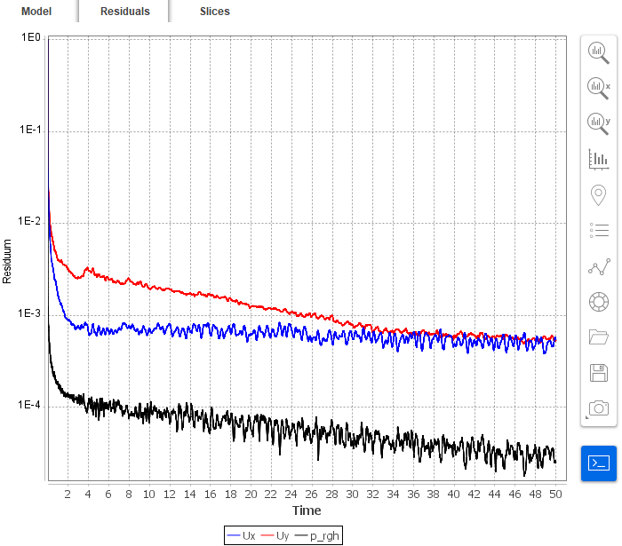
32. Residuals
When the calculation is finished we should see a similar residual plot.
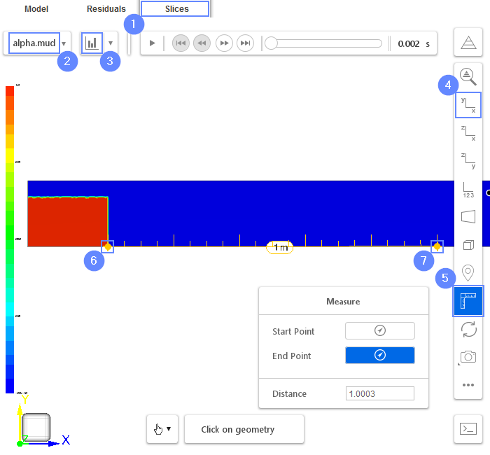
33. Results - Slice (I)
Slices tab appears next to Residuals. Under this tab, we can preview results on the defined slice plane. The results preview is available during the calculation and we can track it on a regular basis. The newly calculated time step will be actualized automatically as long as the time selector points to the latest time step.
We would like to check the time when mud moves 1 meter from the initial position. For this purpose, we will use measurement tools and observe the movement of the mud.
- Switch to Slice tab
- Choose \(\alpha_{mud}\) field to display the mud phase
- Click Adjust range to data
- Set the XY orientation by clicking Viev XY
- Select Measure Distance from right panel
- Hold CTRL key and click the mesh at the lock gate to choose Start Point
- Hold CTRL key and click the mesh at a distance one meter from the lock gate to choose End Point
34. Results - Slice (II)
- Play with animation buttons to view the results of the analysis. Try to measure the time when the front of the current reaches a distance of 1 meter from the lock gate.
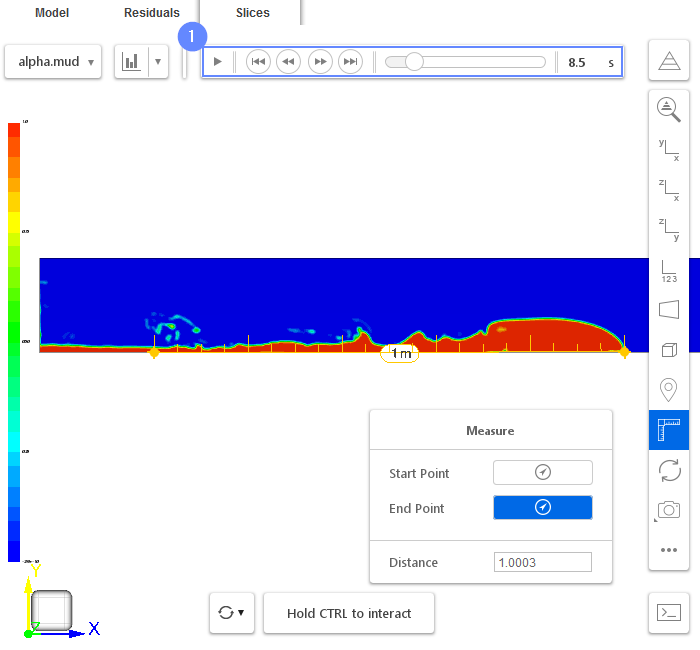
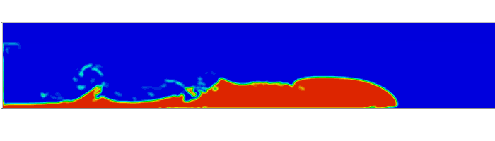
35. Final Results
Experimental data shows that the front of the current reaches a distance of 1m after 8.9s. It is slightly slower than the simulation results which is equal to 8.5s.