3. Create Case
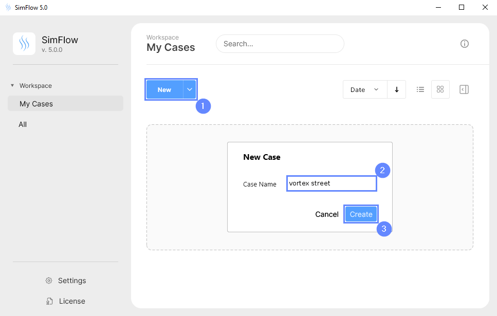
Open SimFlow and create a new case named vortex street
- Click New
- Provide name vortex street
- Click Create to open a new case
4. Create Geometry Parameters
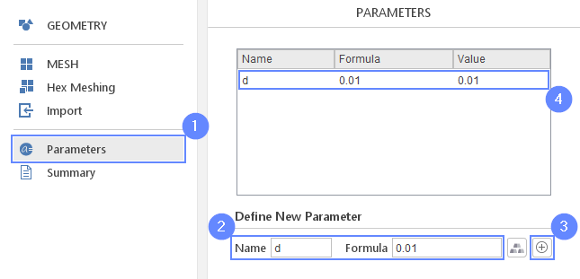
We will be using parameters extensively during this simulation. Therefore, we will add d parameter denoting cylinder diameter.
- Go to Parameters panel
- Define the new parameter
Named
Formula0.01 - Click Enter or Create Parameter button
- The newly created parameter will be shown in the parameters list.
5. Create Geometry - Cylinder
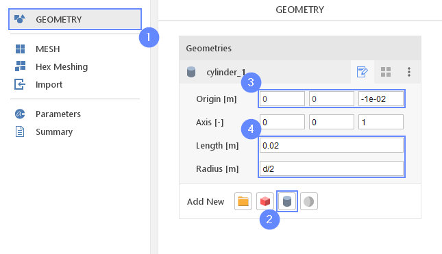
By using the d parameter, we will create a cylinder geometry. The cylinder will be used as an obstacle in the flow path.
- Go to Geometry panel
- Select Create Cylinder
- Set the origin:
Origin \({\sf [m]}\)00-1e-02 - Set the cylinder dimensions:
Length \({\sf [m]}\)0.02
Radius \({\sf [m]}\)d/2
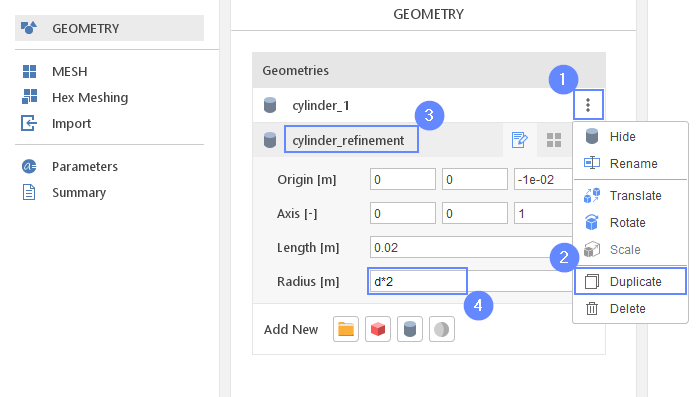
6. Create Geometry - Cylinder Refinement
For better flow prediction in the region near and downstream of the cylinder, we will refine the mesh. For this purpose, we will create refinement geometry.
- Expand options list for cylinder_1
- Select duplicate
- Change geometry name from cylinder_2 to cylinder_refinement
(double click to edit name and press Enter to confirm) - Change the cylinder radius to
Radius \({\sf [m]}\)d*2
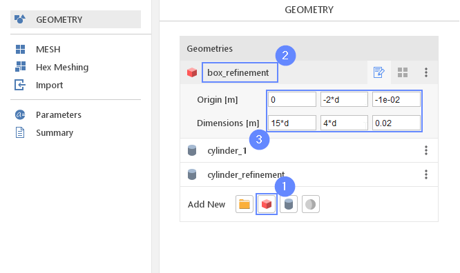
7. Create Geometry - Box Refinement
- Select Create Box
- Change geometry name from box_1 to box_refinement
- Set the origin and box dimensions
Origin \({\sf [m]}\)0-2*d-1e-02
Dimensions \({\sf [m]}\)15*d4*d0.02
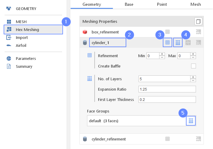
8. Meshing Parameters - Cylinder
Set the meshing parameters for the cylinder geometry. This geometry will be used as a wall, therefore we will additionally enable the boundary layer option.
- Go to Hex Meshing panel
- Select cylinder_1
- Enable Mesh Geometry
- Enable Create Boundary Layer Mesh
- Make sure that Create Boundary Layer On This Group options is pressed
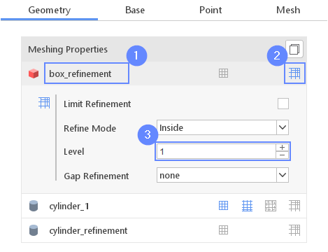
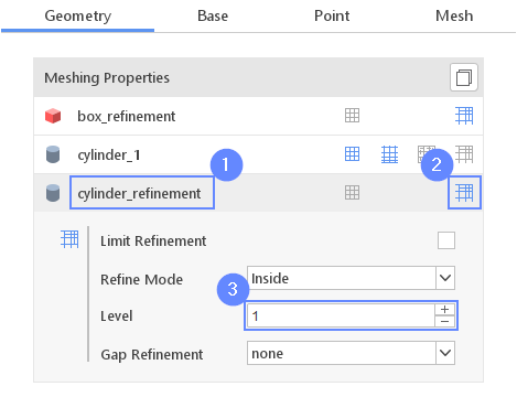
9. Meshing Parameters - Box Refinement
The box_refinement and cylinder_refinement geometries should be used only for marking refinement zones. Set the proper parameters for the refinement regions.
- Select box_refinement from the list
- Enable Refine Geometry
- Set the refinement Level to 1
10. Meshing Parameters - Cylinder Refinement
- Select cylinder_refinement from the list
- Enable Refine Geometry
- Set the refinement Level to 1
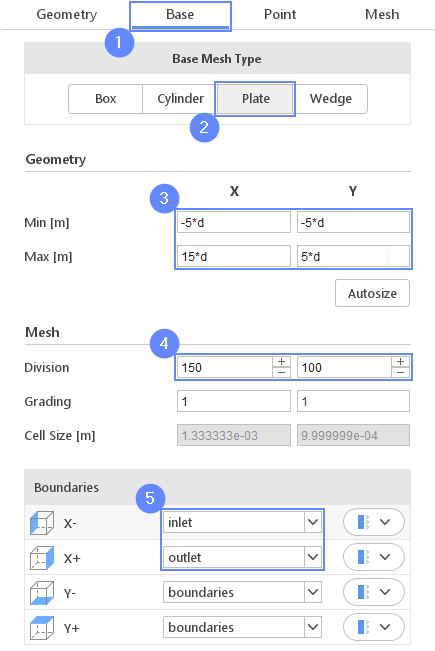
11. Base Mesh
We will define the base mesh now. Our simulation will be limited to a 2D flow. This can be accomplished by choosing the Plate type as the background mesh. We will use predefine parameter d to define the outer flow domain.
- Go to Base tab
- Select the Plate as a Base Mesh Type
- Set the size of base mesh
\(\;\)X \(\quad\)Y\(\quad\)
Min \({\sf [m]}\)-5*d-5*d
Max \({\sf [m]}\)15*d5*d ` - Define the number of divisions
Division150100 - Change the following boundary names accordingly
X- inlet
X+ outlet
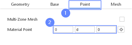
12. Material Point
Material Point tells the meshing algorithm on which side of the geometry the mesh is to be retained. Since we are considering flow outside the cylinder we can use predefined parameter d to specify the desired point location.
- Go to Point tab
- Specify location inside base mesh but outside cylinder_1 geometry
Material Point0d0
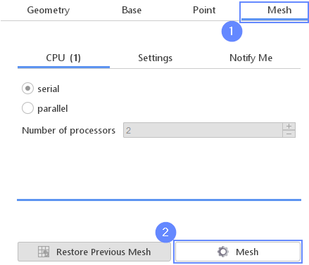
13. Start Meshing
Everything is now set up for meshing
- Go to Mesh tab
- Press the Mesh button to start meshing process
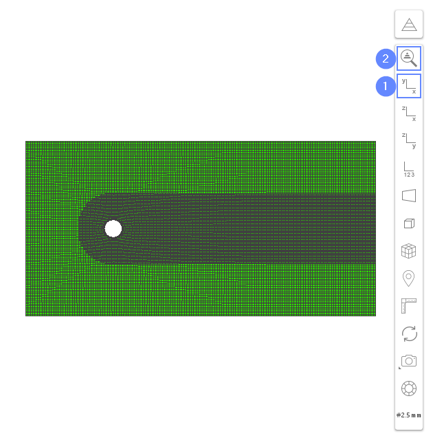
14. Mesh
After the meshing process is finished the mesh should appear in the graphics window.
- Set the XY orientation View XZ
- Click Fit View
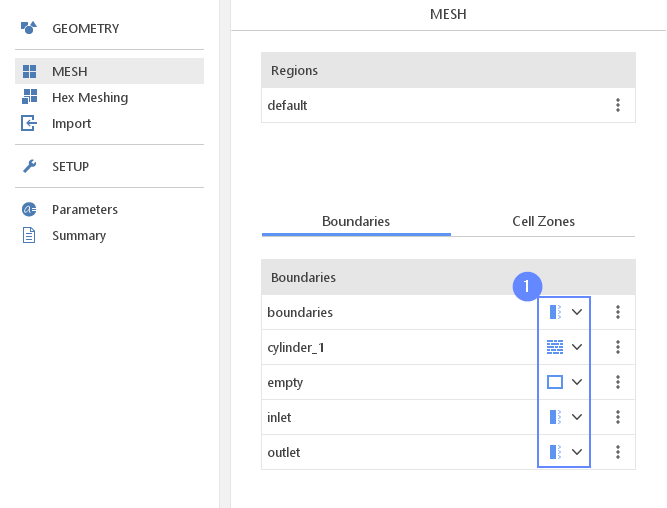
15. Boundaries
- Define boundary types accordingly
boundaries patch
cylinder_1 wall
empty empty
inlet patch
outlet patch
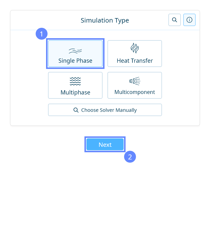
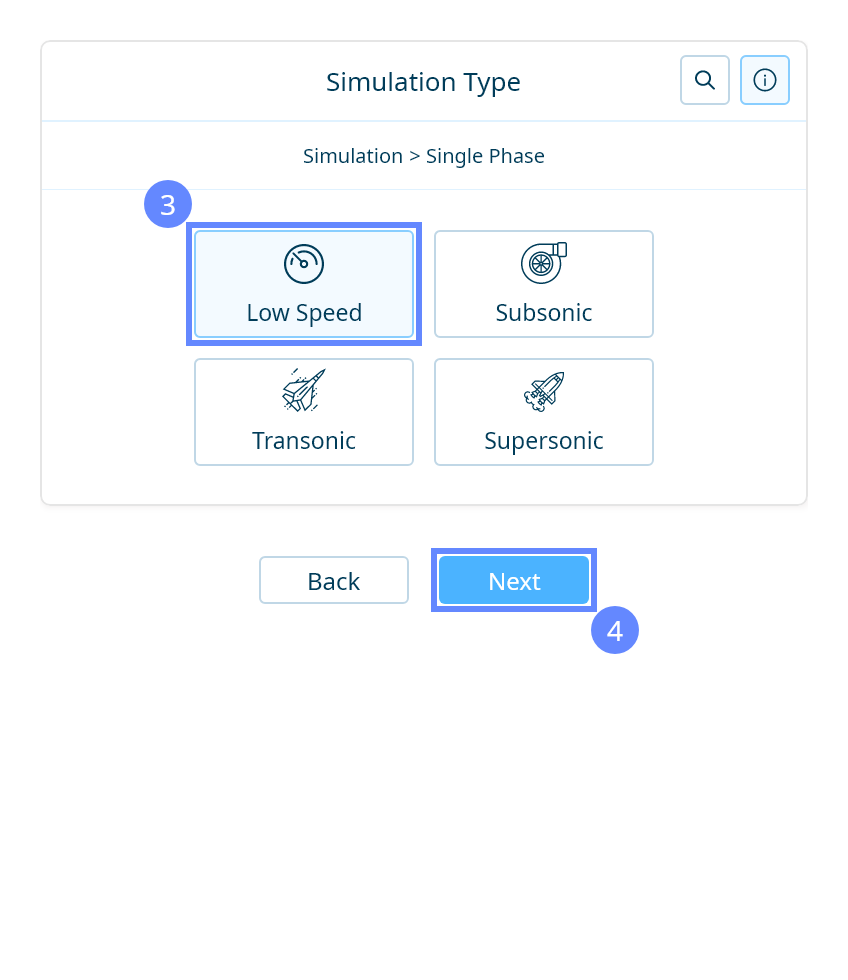
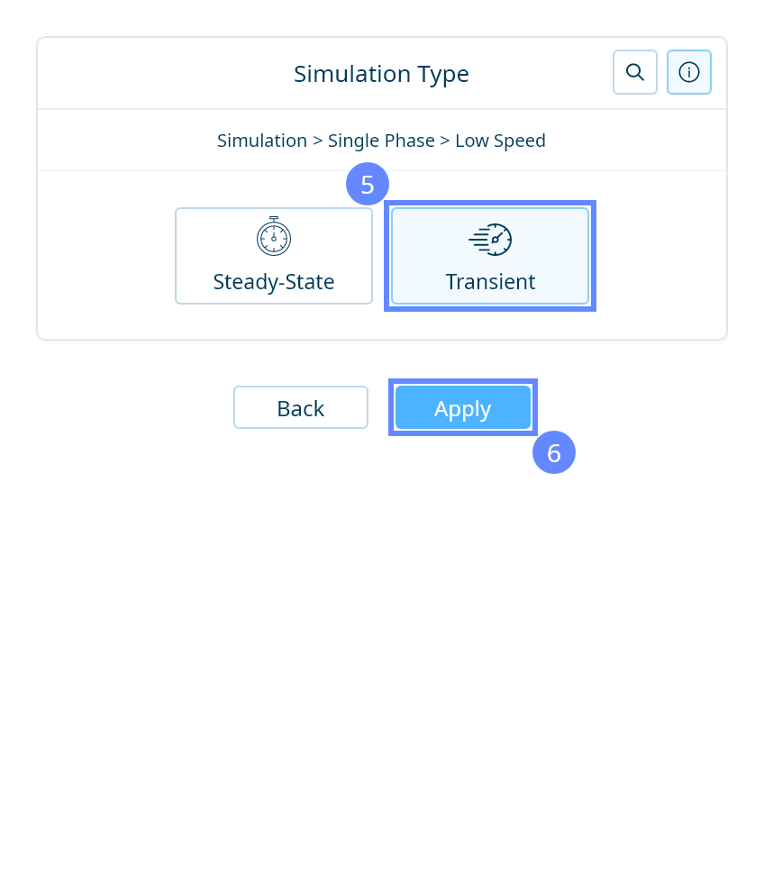
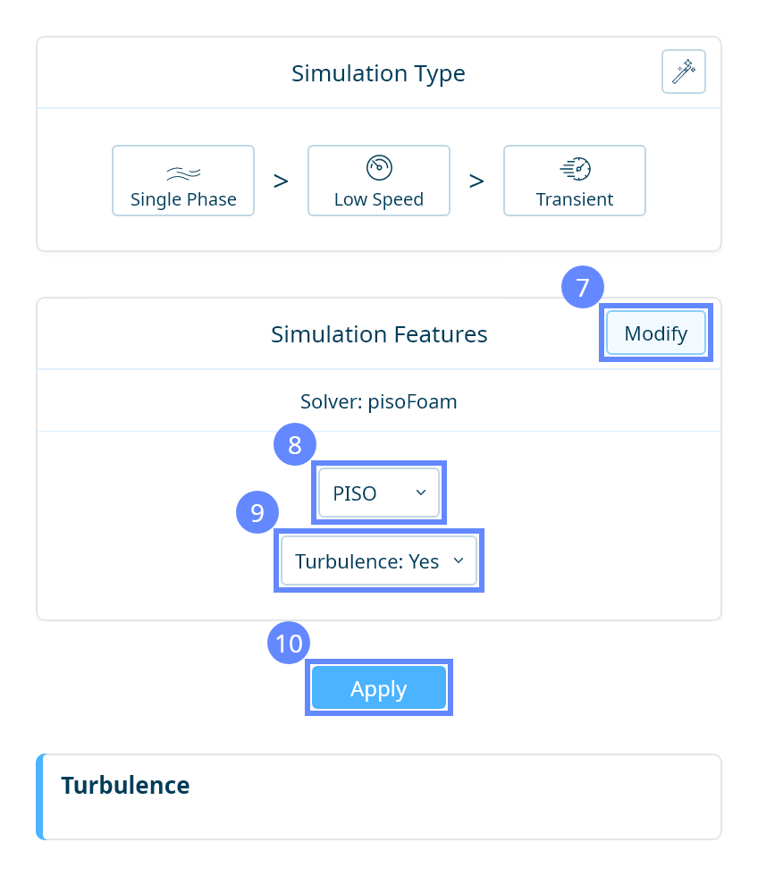
16. Simulation Type
We want to analyze the vortex shedding behind a cylinder. For this purpose, we will use a single phase, transient, incompressible flow simulation using the PISO algorithm.

17. Create Simulation Parameters (I)
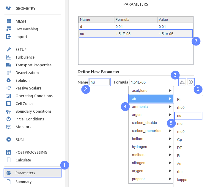
We need to define a few parameters that will be used in the simulation setup. First one is a kinematic viscosity of the air nu . This value can be found in Material Database .
- Go to Parameters panel
- Define new parameter Name as nu
- Click on Select Material Property
- Extend air property list
- Select kinematic viscosity nu
- Click enter or Create Parameter button
- The newly created parameter will be shown in the parameters list.
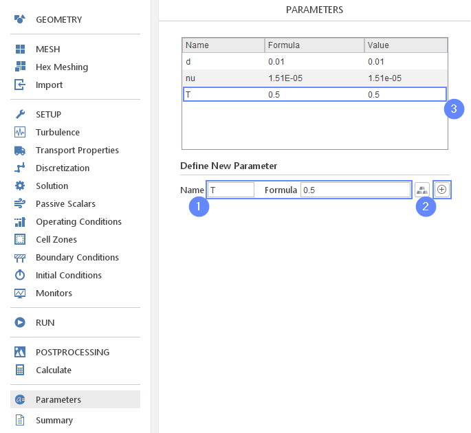
18. Create Simulation Parameters (II)
Also, we will define the flow velocity and period of the vortex shedding, which can be defined as the time interval between the appearance of successive vortices. Both properties depend on each other while the relationship can be described empirically Karman vortex street . By using this fact, we will calculate the velocity value as a function of the vortex shedding period. At the end, we will compare the assumed time to simulation results.
- Define the period of vortex shedding
NameT
Formula0.5 - Click enter or Create Parameter button
- The newly created parameter will be shown in the parameters list.
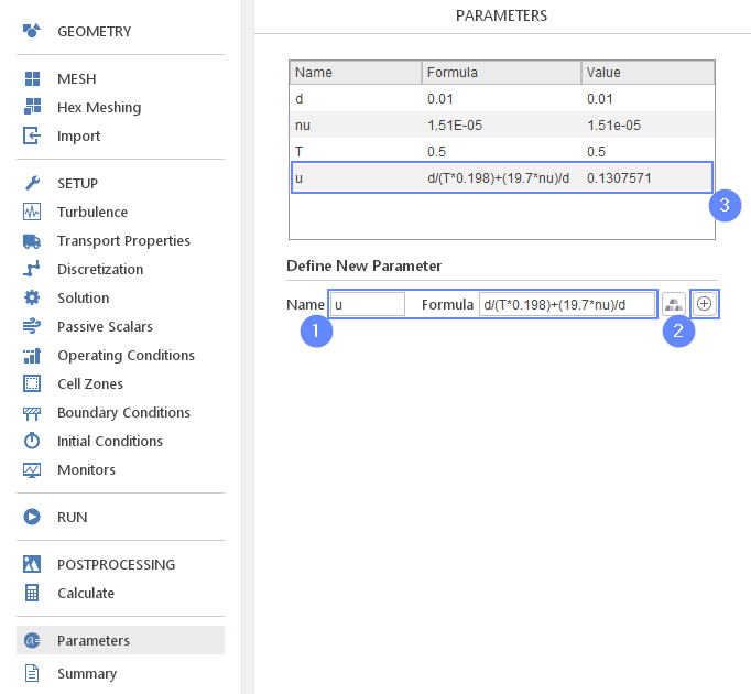
19. Create Simulation Parameters (III)
Define the velocity magnitude parameter.
- Define the velocity parameter
Nameu
Formulad/(T*0.198)+(19.7*nu)/d - Click enter or Create Parameter button
- The newly created parameter will be shown in the parameters list.
According to empirical equation flow velocity should be equal 0.13 m/s
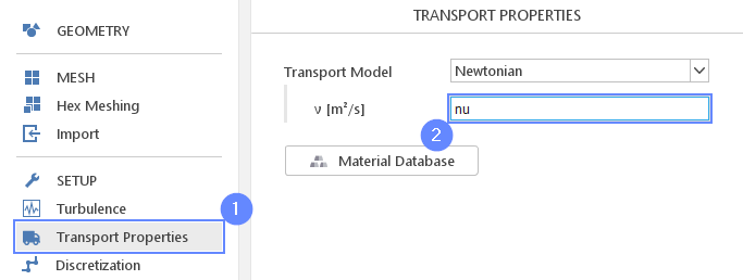
20. Transport Properties
Change kinematic viscosity to the parametrized value nu
- Go to Transport Properties panel
- Set the kinematic viscosity \(\nu \; [m^2/s]\) to nu
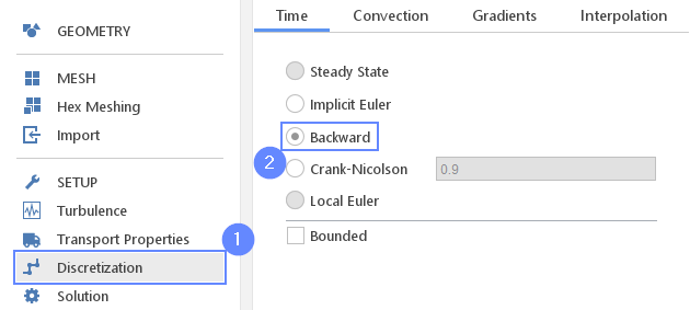
21. Discretization - Time
For the better accuracy of our solution, we will use the 2nd order scheme for the discretization of the time derivatives.
- Go to Discretization panel
- Select Backward
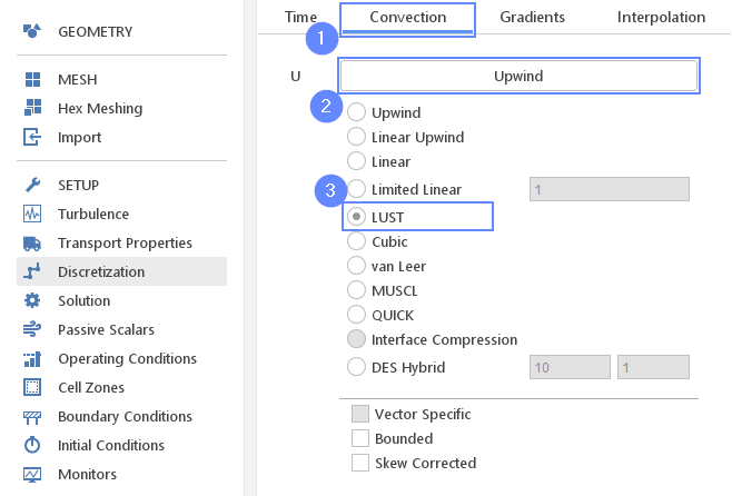
22. Discretization - Convection
Change velocity discretization to the LUST scheme. It is a second-order spatial discretization scheme that allows to reduce the numerical diffusion.
- Go to Convection tab
- Click on default scheme Upwind
- Select LUST
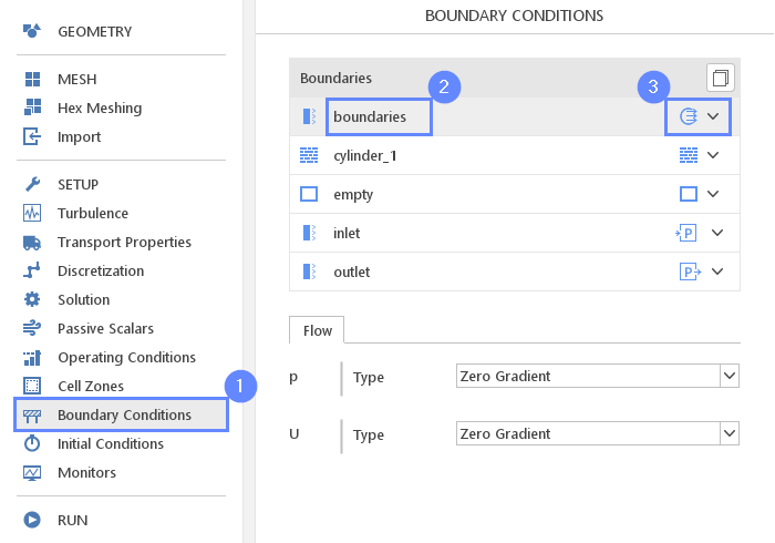
23. Boundary Conditions - Boundaries
The sides of the domain will be set to the Outflow character which should adjust velocity and pressure at the boundaries to the flow inside the domain.
- Go to Boundary Conditions panel
- Select boundaries
- Set the Outflow character
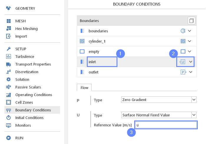
24. Boundary Conditions - Inlet
Now we will apply the computed velocity parameter to the inlet boundary.
- Select inlet boundary
- Set the Velocity Inlet character
- Set the velocity Reference Value [m/s] to u parameter
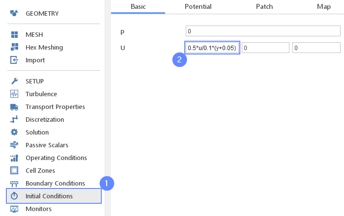
25. Initial Conditions
Before we start simulation we need to define the initial state. We will specify a linear velocity profile that changes from zero at the bottom of the domain to 50% of the velocity magnitude. We will use the profile to boost instabilities appearance by introducing flow asymmetry at the initial state. The von Karman instabilities under certain conditions would appear spontaneously, but it might require a longer time for instabilities to arrive if we would start with a uniform velocity.
- Go to Initial Conditions panel
- Set the initial velocity
U0.5*u/0.1*(y+0.05)00
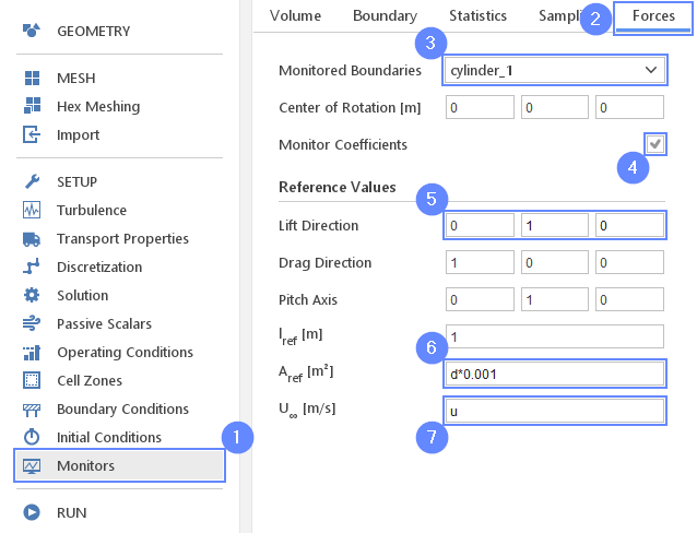
26. Monitors - Forces
In order to track periodic features in the flow, we will use the force monitor. We will observe drag and lift on the cylinder boundary.
- Go to Monitors panel
- Switch to Forces tab
- Expand Monitored Boundaries list and check cylinder_1
- Check Monitor Coefficients option
- Set Lift Direction vector along Y axis
Lift Direction010 - Set the reference area \(A_{ref} \; [m^2]\) to d*0.01
- Set the free stream velocity \(U_{\infty} \; [m/s]\) to u
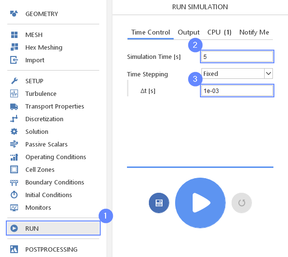
27. Run - Time Control
Before running computations adjust the time controls in order to capture appropriate time scales of the flow features.
- Go to RUN panel
- Set the Simulation Time [s] to 5
- Set the Time Stepping \(\Delta t \; [s]\) to 1e-03
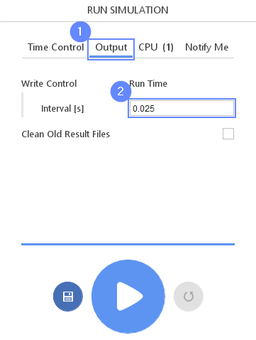
28. Run - Output
We will write the results in the interval of 0.025 seconds (every 25 steps).
- Switch to Output tab
- Set the Interval [s] to 0.025
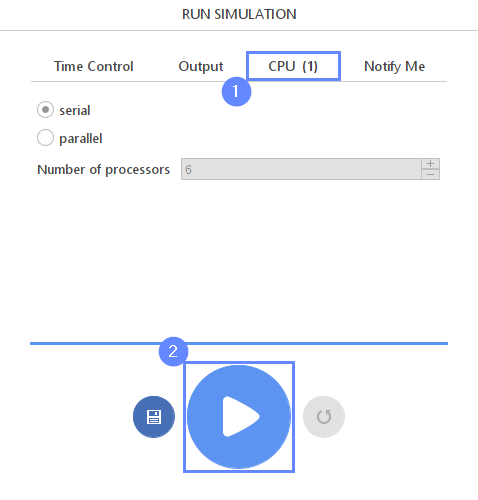
29. Run - CPU
To speed up the calculation process, take advantage of parallel computing and increase the number of CPUs based on your PC’s capability. The free version allows you to use only one processor (serial mode). To get the full version, you can use the contact form to Request 30-day Trial
Estimated computation time for serial mode: 8 minutes
- Switch to CPU tab
- Click Run Simulation button
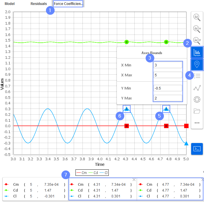
30. Results - Force Coefficients
We are going to read the period of the vortex shedding. To do so we will read the time of two last extrema for the Cl coefficient. The difference between them gives us the periods of the vortex shedding.
- Switch to Force Coefficient tab
- Click on the Adjust Axes
- Set the Axes Bounds
X Min3
X Max5
Y Min-0.5
Y Max2 - Check the Lookup Data button
- Click on the last Cl extremum to read the coordinates
- Click on the one before last Cl extremum to read the coordinates
- Selected points are listed below the chart. Report time values that we will use later.
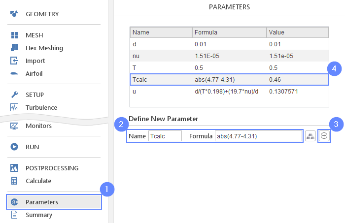
31. Output Parameters - Tcalc
Finally, we will compare the assumed period of the vortex shedding with the result of our simulation. The assumed period is 0.5 second, while the simulation one can be computed as a time difference between the occurrences of the two last Lift Coefficient maxima.
- Define the Tcalc parameter
NameTcalc
Formulaabs(4.77-4.31) - Add a new parameter
- Parameter will be added to the list above
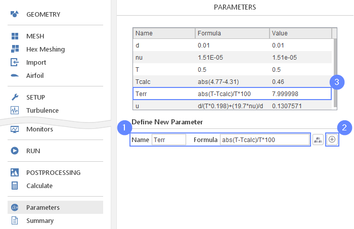
32. Output Parameters - Terr
Additionally, we will present the result as a relative error between the expected value and obtained one.
- Define the Terr parameter
NameTerr
Formulaabs(T-Tcalc)/T*100 - Add a new parameter
- Parameter will be added to the list above. Read the value of Terr
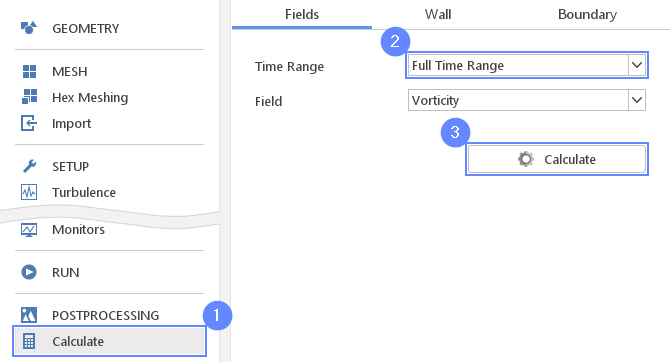
33. Calculate Vorticity
The vorticity is not being computed by default during solver computations. In order to visualize it, we will compute the vorticity variable by using already existing data.
- Go to Calculate panel
- Select Full Time Range
- Click on Calculate
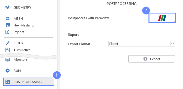
34. Postprocessing - ParaView
Start ParaView to visualize the vorticity field.
- Go to POSTPROCESSING panel
- Click on Run ParaView
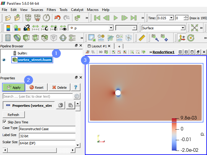
35. ParaView - Load Results (I)
Load the results into the program.
- Select vortex_street
- Click Apply to load results into ParaView
- After loading results they will be shown in the 3D graphic window
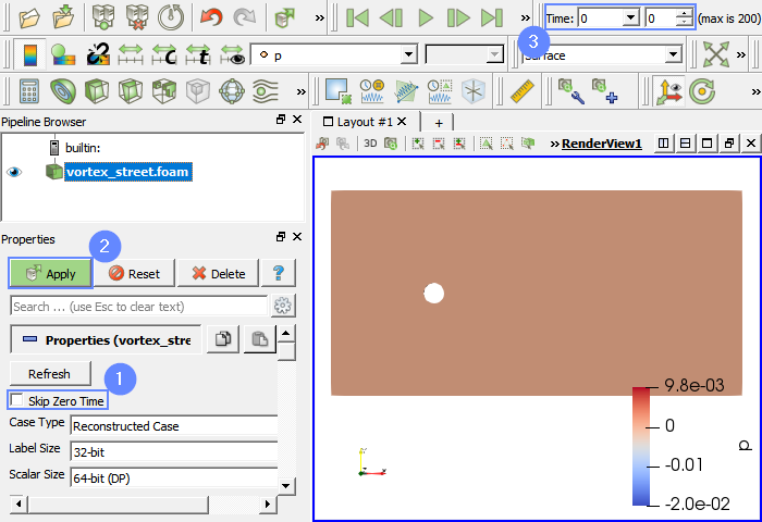
36. ParaView - Load Results (II)
ParaView skips the initial point by default, therefore we need to add the zero time point to simulation.
- Uncheck Skip Zero Time
- Click Apply
- Set the time or time step to 0
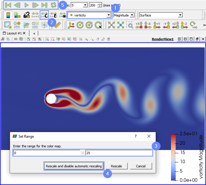
37. ParaView - Vorticity
We will look at the vorticity contour map. Change the scale range parameters to improve flow features visibility.
- Select vorticity from the list
- Click Rescale to Custom Data Range
- Set the range for the color map from 0 to 25
- Click Rescale and disable automatic rescaling
- Play with an animation buttons to track the results of analysis.