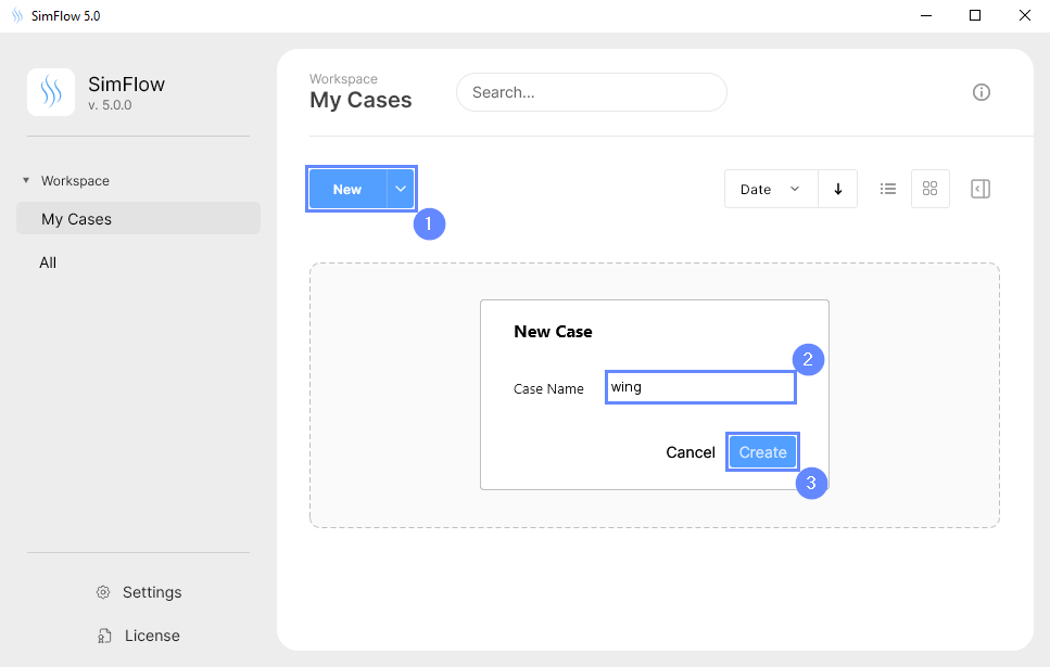
3. Create Case
Open SimFlow and create a new case named wing
- Click New
- Provide name wing
- Click Create to open a new case
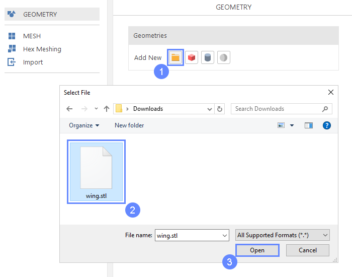
4. Import Geometry
Firstly, we need to Download GeometryWing
- Click Import Geometry
- Select geometry file wing.stl
- Click Open
5. Imported Geometry Units
The STL format does not contain the unit information which are defined during the geometry export. If we do not know the exported unit, we can estimate it based on the total size of the model. It is displayed next to Geometry size label. In our case, the default unit meter is correct.
- To confirm default unit meter, press OK

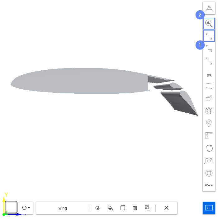
6. Geometry - Wing
After importing geometry, it will appear in the 3D window.
- Set the XY orientation View XY
- Click Fit View to fit geometry in the view
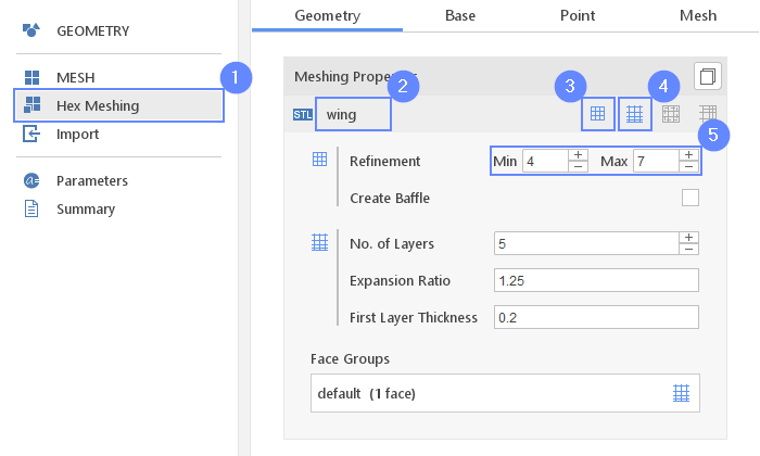
7. Meshing Parameters - Wing
In order to create the mesh, we need to specify geometry options for the meshing process. We will increase mesh resolution near the wing surface.
- Go to Hex Meshing panel
- Select wing
- Enable Mesh Geometry
- Enable Create Boundary Layer Mesh
- Set Refinement to Min 4 Max 7
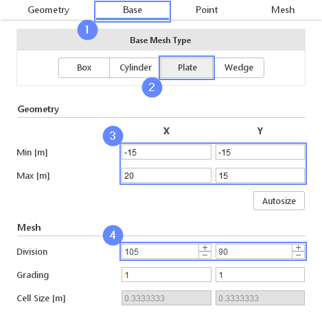
8. Base Mesh - Domain
Our simulation will be limited to a 2D flow. This can be accomplished by choosing the Plate type as the background mesh.
- Go to Base tab
- Select Plate as a Base Mesh Type
- Define minimum and maximum extend
Min \({\sf [m]}\)-15-15
Max \({\sf [m]}\)2015 - Set the division of the base mesh
Division10590
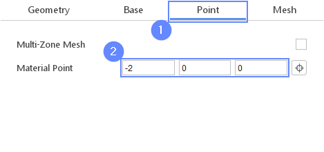
9. Material Point
Material Point tells the meshing algorithm on which side of the geometry the mesh is to be retained. Since we are considering flow around the wing we need to place the material point outside the geometry.
- Go to Point tab
- Specify location inside base mesh but outside wing geometry
Material Point-200
You can specify the point location from the 3D view. Hold the CTRL key and drag the arrows to the destination.
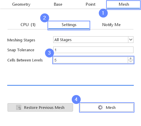
10. Start Meshing
We can define the count of the buffer cells between refinement levels. This parameter determines the width of the transition zone between refined and background mesh. A higher value of this parameter will increase the overall cells count.
- Switch to Mesh tab
- Go to Settings
- Change Cells Between Levels to 5
- Start the meshing process with Mesh button
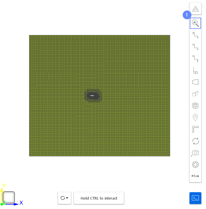
11. Mesh
After the meshing process is finished the mesh should appear in the graphics window.
- Click Fit View to fit mesh in the view
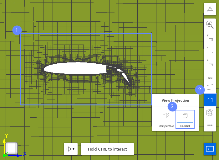
12. Examine Mesh
For further examination, we should zoom in to see the refinement mesh. Additionally, we can switch projection view from perspective to parallel as the parallel view is more appropriate for visualizing 2D objects.
- Zoom in the mesh - use the Scroll Wheel or drag mouse with RMB (right mouse button) pressed
- Click on Change View Projection
- Select Parallel view
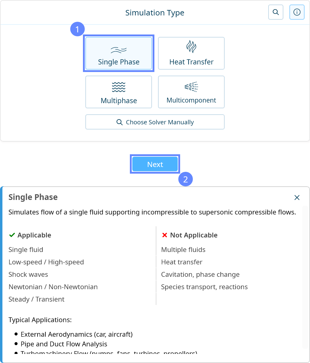
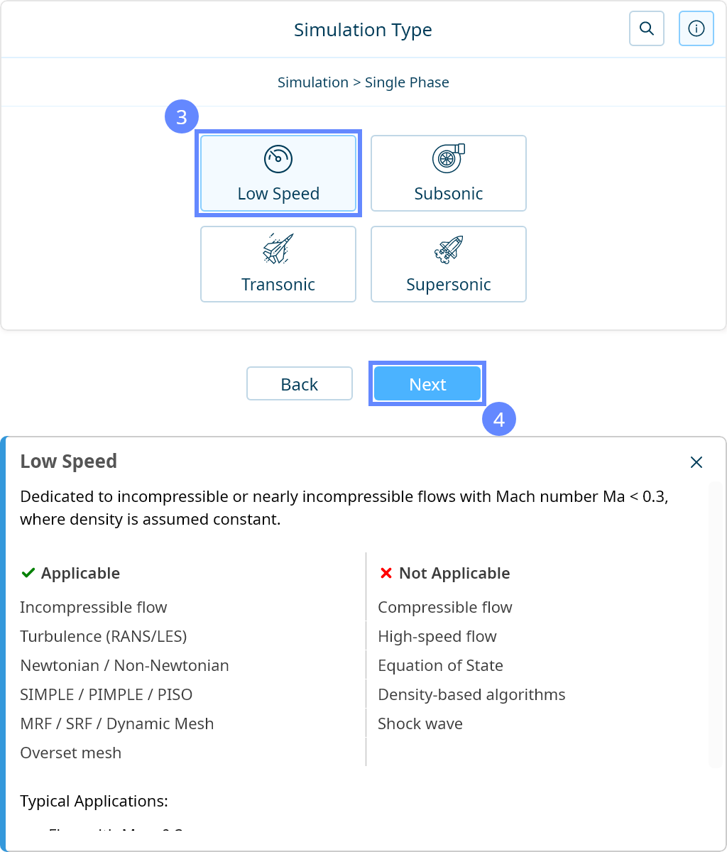
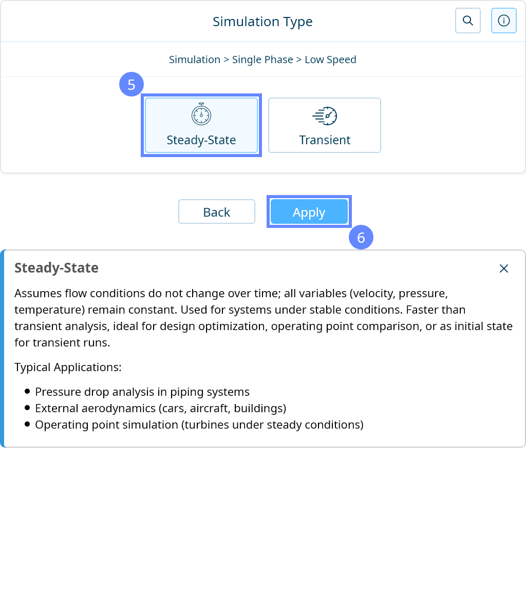
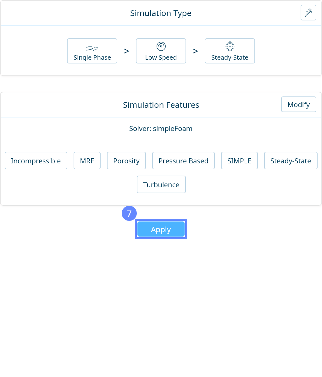
13. Simulation Type
We want to analyze the turbulent flow around the airfoil. For this purpose, we will use a single-phase, steady-state simulation of incompressible turbulent flow.

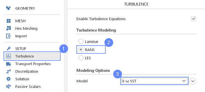
14. Turbulence
For the purpose of this tutorial, we will simulate the turbulence phenomenon using the \(k{-}\omega \; SST\) model.
- Go to Turbulence panel
- Select RANS turbulence formulation
- Select \(k{-}\omega \; SST\) model
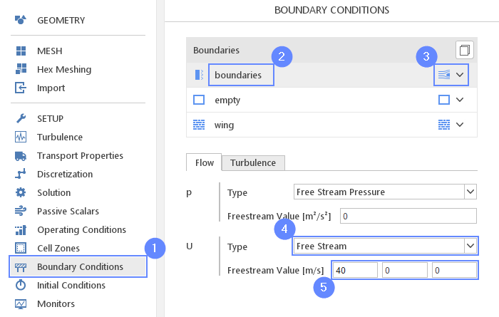
15. Boundary Conditions - Boundaries (Flow)
The domain has only one external boundary. We will use the Free Stream character type to model the far field conditions. The flow will be aligned with the x-axis.
- Go to Boundary Conditions panel
- Select boundaries
- Set the Free Stream character
- 5 Change the velocity type and value accordingly
U TypeFree Stream
U Freestream Value \({\sf [m/s]}\)4000
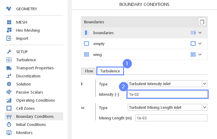
16. Boundary Conditions - Boundaries (Turbulence)
Additionally, to flow conditions, we will modify default free stream turbulence properties.
- Switch to Turbulence tab
- Set the k Intensity [-] to 1e-02
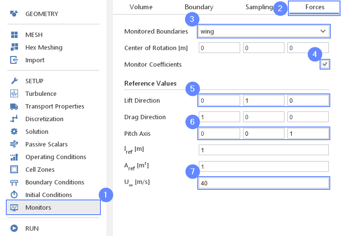
17. Monitors - Forces
In order to measure aerodynamic forces, we will use the force monitor. We will observe drag and lift force coefficients on the aerofoil boundary.
- Go to Monitors panel
- Switch to Forces tab
- Expand Monitored Boundaries list and check wing
- Check Monitor Coefficients option
- Set lift direction vector along Y axis
Lift Direction010 - Set pitch axis vector along Z axis
Pitch Axis001 - Set the reference velocity
\(U_{\infty}\) \({\sf [m/s]}\)40
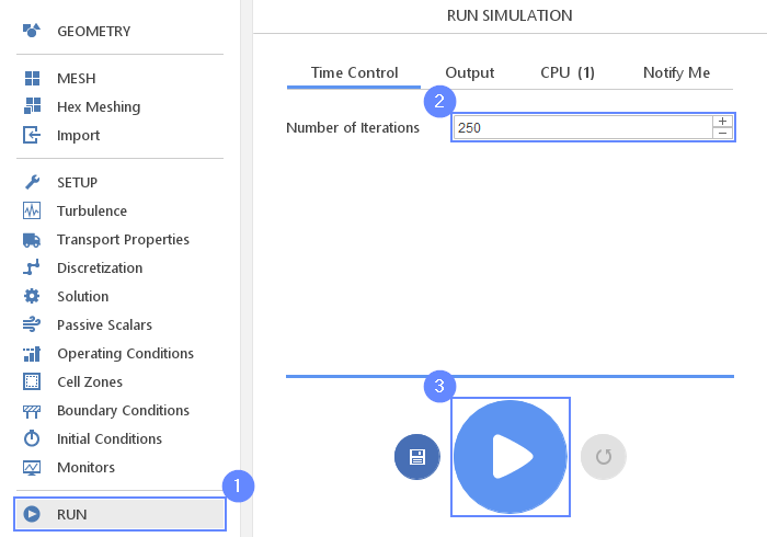
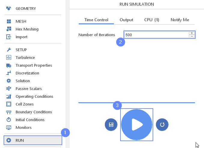
18. Run - Time Control
- Go to RUN panel
- Set the maximal Number of Iterations to 250
- Click Run Simulation button
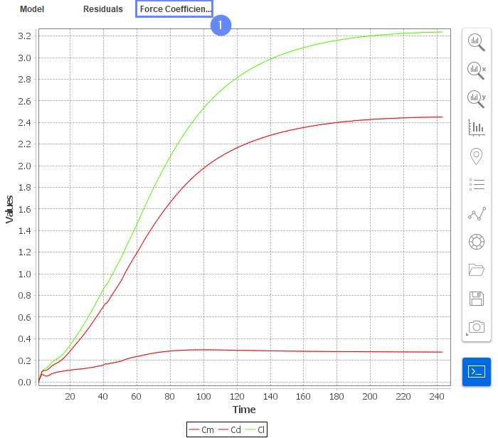
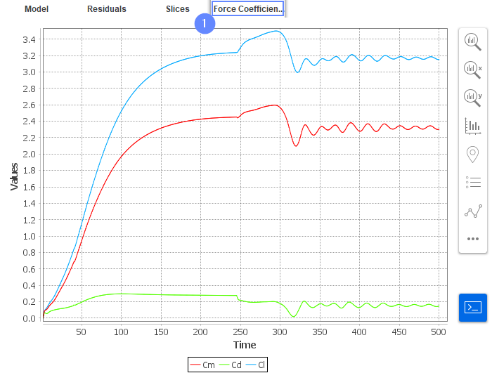
19. Results - Force Coefficient
During the simulation, we can observe whether forces on the wing stabilize which will mean that our simulation converges
- Go to Force Coefficient tab
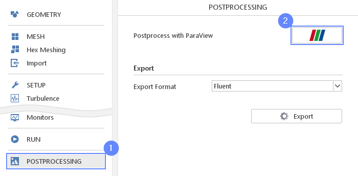
20. Postprocessing - ParaView
After the computation is finished we can do a comprehensive visualization of our results with ParaView.
- Go to POSTPROCESSING panel
- Click on Run ParaView
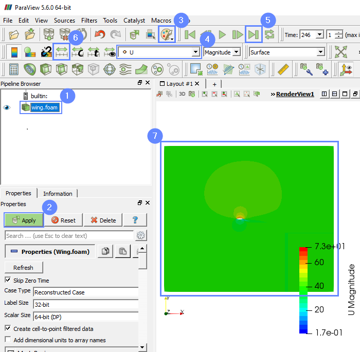
21. ParaView - Load Results
After opening the ParaView, we need to load the simulation results from SimFlow.
- Select your case wing.foam
- Click Apply to load results into ParaView
- Click Load a color palette and choose White Background
- Select the velocity U from the list
- Load the latest results by clicking Last Frame icon
- Click Rescale to data range
- After loading results they will be shown in the 3D graphic window. Your default color map may be different than the one below. Go to the next slide and choose an appropriate preset.
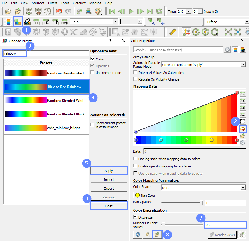
22. ParaView - Choose Preset
- Click Edit Color Map from the menu placed on the left side
- Select Choose Preset from the Color Map Editor placed by default on the right side of the ParaView
- Search rainbow
- Choose Blue to Red Rainbow preset
- Apply changes
- Close Choose Preset window
- Set Number of Table Values to 20
- Click Save current color map settings values as default for all arrays
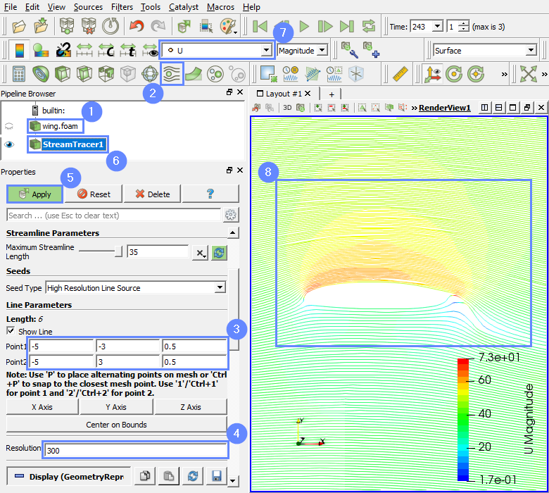
23. ParaView - Streamlines
We can visualize the flow by displaying the streamlines.
- Select your case wing.foam
- Select Stream Tracer from top menu
- Set the start point and end point of the streamline source
Point1-5-30.5
Point2-530.5 - Set the number of streamlines
Resolution300 - Click Apply
- Select StreamTracer1
- Select the velocity U from the list
- Zoom in to the wing profile
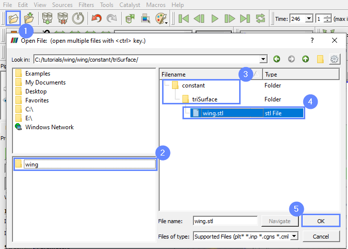
24. ParaView - Import Wing Geometry (I)
To display the wing geometry with the streamlines, we need to read the geometry file to the ParaView.
- Select Open from top menu
- From the bottom left menu select wing folder
- From the right menu open constant and than triSurface folder
- Select wing.stl
- Press OK
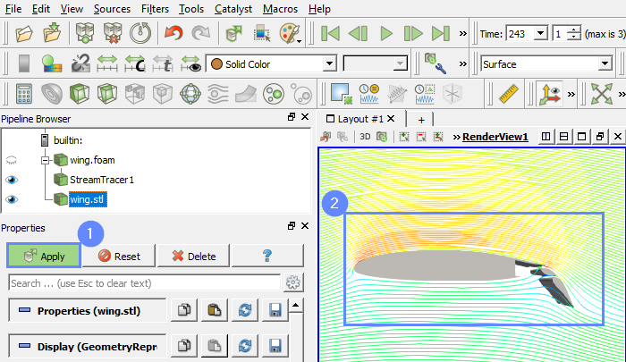
25. ParaView - Import Wing Geometry (II)
Confirm default properties and display geometries with streamlines.
- Click Apply to load geometry
- After loading geometry, it will be shown in the 3D graphic window
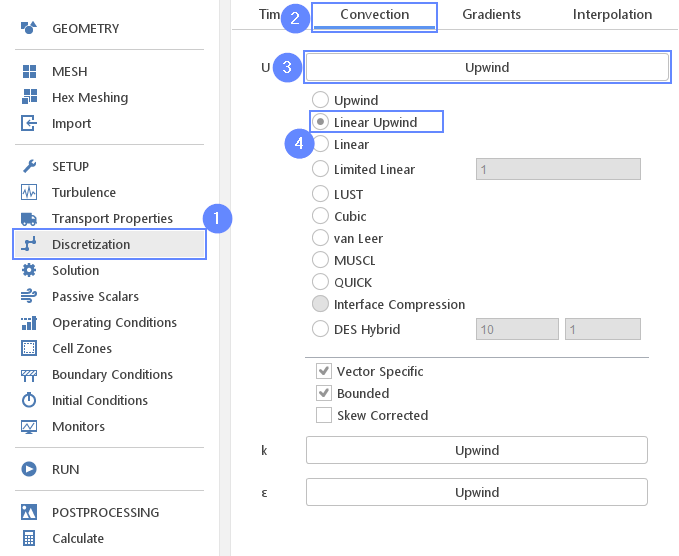
26. Discretization - Convection
After preliminary calculation, we will continue with a more accurate algorithm. Go back to the Simflow but do not close the ParaView yet. Change velocity discretization to the Linear Upwind scheme. This will decrease numerical diffusion affecting the results.
- Go to Discretization panel
- Switch to Convection tab
- Click on Upwind to extend the list
- Select Linear Upwind
27. Run - Continue Simulation
- Go to RUN panel
- Increase the Number of Iterations to 500
- Click Continue Simulation button
Estimated computation time: 1 minute
28. Force Coefficient
You can observe in the Force Coefficient plot that after switching to second-order the coefficients started to oscillate.
- Switch tab to Force Coefficient
29. ParaView - Reload the results
Switch window to ParaView once again. To read newly calculated steps we need to reload the results.
- Click Refresh
- Click Last Frame to display the latest results
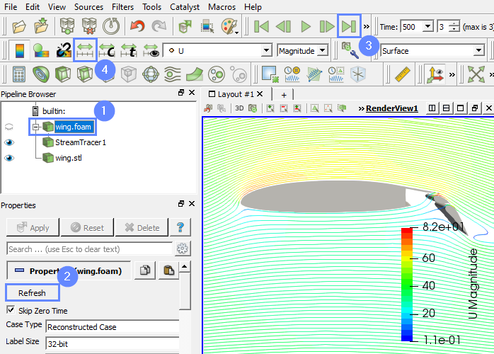
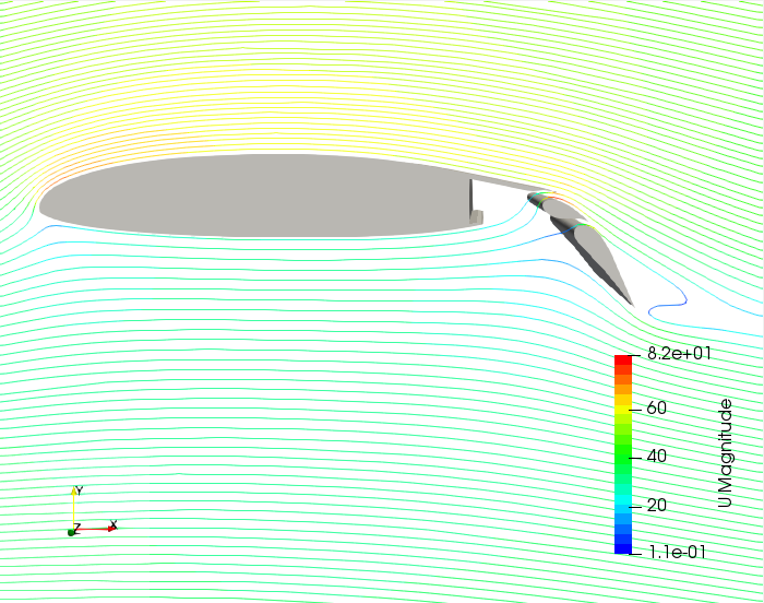
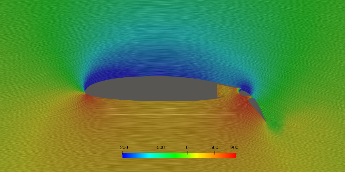
30. ParaView - Streamlines Results
Finally, we can see the results in the 3D window. We observe the flow separation on the second flap. This separation is the cause of the flow instability that we have observed as oscillating values of the force coefficients.