Buice-Eaton 2D diffuser - CFD Simulation SimFlow Validation Case

Flow separation is often met in many engineering problems including diffusers, turbomachinery and aircrafts. What is interesting, the flow separation and reattachment is still a challenging task for many CFD codes.

In this study we will consider a well-known validation case of asymmetric two-dimensional diffuser, also known as a Buice-Eaton 2D diffuser. The flow through such a diffuser includes three important features:

We will model two-dimensional, incompressible, turbulent, fully-developed flow with Reynolds number of 20 000 based on the centreline velocity and the channel height. The simulation results will be compared to the experimental data by [Buice and Eaton]. The same modelling strategy was incorporated as in [numerical study of NASA].

The geometry of the asymmetric diffuser is presented in Figure 1. The x-axis is taken along the main flow direction and y-axis in straight-wall normal direction. The origin of the x-axis is at the intersection of the tangents to the straight and inclined wall (see the detail in Figure 1). The origin of the y-axis is located at the bottom wall of the downstream channel. The height of the inflow domain \(H\) is \(0.015 \; m\).

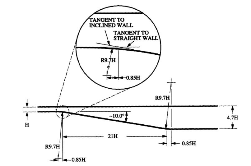
Figure 2 presents the extended geometry of the diffuser - inlet and outlet. The reason why the inlet is extended (110H) is the fact that the flow must be fully-developed. We have two options. First, we can run channel flow simulation and then export the proper boundary conditions. Second, we can design the geometry in such a way that inlet is sufficiently long to create the turbulent, fully-developed flow. The second approach was chosen in this study. The same procedure was applied for the outlet.

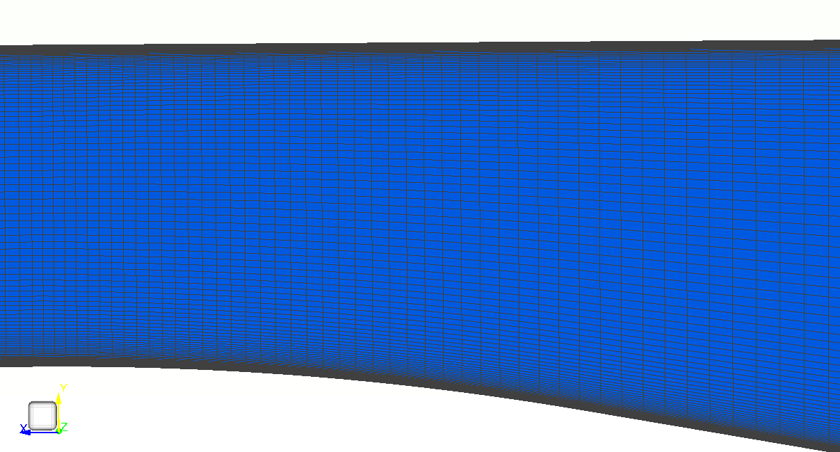
In the [numerical study of NASA] the numerical mesh with \(y^+ < 1\) was used. The mesh is published, therefore we imported that mesh to SimFlow to be able to compare the results and exclude influence of the mesh. NASA provided only the surface mesh which had to be extended in z direction, by means of extrude2DMesh utility, which is a part of OpenFOAM. The grid in the region of a channel with smooth transition to downstream part is shown in Figure 3. The maximum value of \(y^+\) reported by SimFlow is 0.259 and the average value is 0.0552. The total mesh size is 66 000 cells.

Steady-state, incompressible simulation was conducted in SimFlow. The incompressible solver (simpleFoam) is using the Semi-Implicit Method for Pressure Linked Equations (SIMPLE) algorithm for solving the flow equations.
The material used in the simulation was air with kinematic viscosity \(\nu=1.51\cdot 10^{-4} \; \frac{m^2}{s}\).
\(k{-}\omega \; SST\) turbulence model was chosen with Low Reynolds formulation (\(y^+ \leq 1\)).

Boundary conditions are summarized in the table below:

We also need to comment on the approach we took to get the solutions and the choice of the boundary conditions. The crucial step was to ensure that the flow at the inlet is turbulent and fully-developed. That is why the inlet was extended significantly. We follow the same approach regarding the boundary conditions as in study of NASA, namely, the flow is pressure driven. At the inlet we assumed the total pressure of \(14.7 \; psi\) (which corresponds to \(101350 \; Pa\)). Then we monitored the center line velocity and controlled it by reducing the backflow static pressure, reaching the final value of \(100975 \; Pa\). Alternatively, we also tested the initial velocity boundary condition (centre line velocity \(22.585 \; \frac{m}{s}\)) with zero gradient at the outlet. The results obtained with the second approach are very similar to the first one.

It is worth noting that for the flow initialization we first calculated laminar flow and then mapped the results to the final solution.

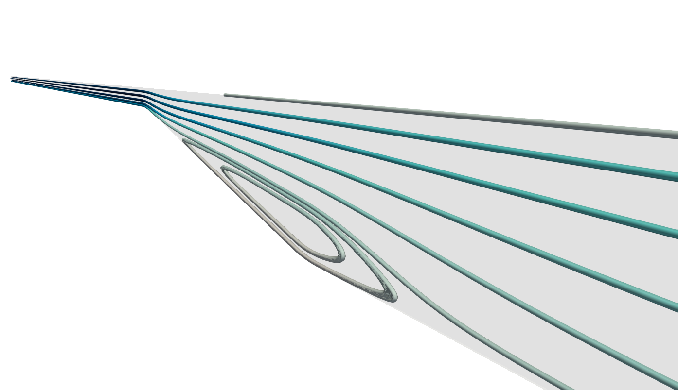
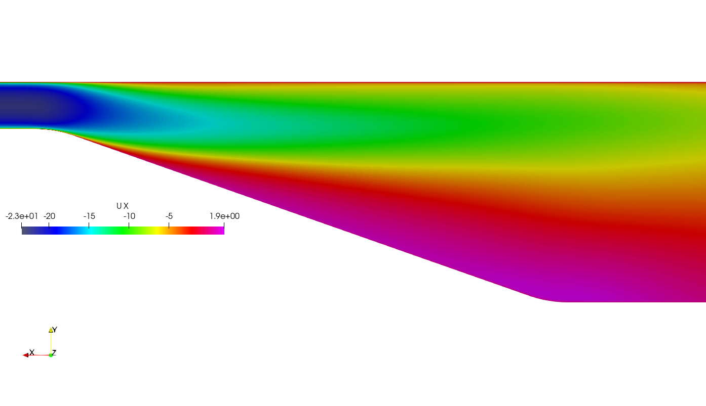
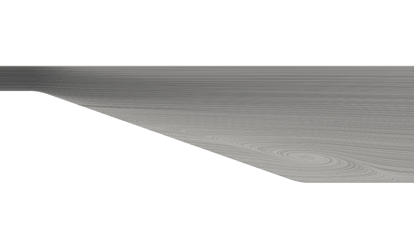
Figure 4 shows the axial velocity contours (x-component of velocity) in the downstream part of the diffuser. Figure 5 represents the recirculation area in the diffuser.

Comparison of velocity profiles between simulation and experimental data are shown in Figure 6, for different sections of the diffuser. The profile \(x/H=-5.82\) represents the fully developed channel flow. For \(x/H\) higher than \(0\) we observe profiles for the downstream part of the diffuser ramp.

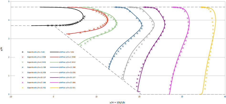
Based on the velocity profiles we can say that \(k{-}\omega \; SST\) turbulence model is able to capture correctly the main features of the flow in the expanding diffuser flow. From the velocity profiles, regions of the reversed flow can be identified. For example we see for \(x/H=27.066\) profile the change of the velocity direction near the bottom wall of the diffuser. One may conclude that still the separation region appears there but definitely ends for \(x/H\) larger than \(30\).

We performed asymmetric diffuser validation with SimFlow. It was shown that the software is perfectly able to capture all the features of the flow. It should be noted that the accuracy of the solution obtained is comparable to results of NASA.

\(k{-}\omega \; SST\) turbulence model is a proper choice for flows including separation and reattachment of the boundary layer. However, it should be noted that proper initialization of the model is necessary to achieve the stability and accuracy of the solution.