(CHT) Conjugate Heat Transfer - Pipe - CFD Simulation SimFlow Validation Case

Interaction between fluids and solids can be found in many engineering applications, for example heat exchangers, car engines, electronics cooling. The speed of fluid, material properties, flow pattern influence the heat exchange which drives the performance of many devices.

The design of such devices is not easy, because analytical prediction of the temperature distribution are limited to some simple cases. To get more detailed understanding of the heat transfer for complicated flow patterns we might use CFD and the special solvers called Conjugate Heat Transfer (CHT) which combine heat transfer in solids (mostly dominated by conduction) with heat transfer in fluids (mostly dominated by convection).

If we consider the heat transfer without any source term or radiation, the remaining options are conduction and convection. For solids, the steady state conduction is expressed by the Fourier’s law:

which means that the heat transfer in a solid body is controlled by a thermal conductivity property (material property) and temperature gradient.

On the other hand, the heat transfer in a fluid can be expressed by the energy equation, which in the simplest case, has the following form:

where \(\rho\) is density, \(C_p\) is the specific heat of the fluid. We can see, that in case of heat transfer in fluids significant role plays also the fluid velocity, which is responsible for heat convection.

In the following article we will present the results of validation of the CHT solver available in SimFlow. The validation case will represent external cooling of a water pipe with a cool air. We will consider the case with free and forced convection. For the both scenarios we will compare simulation results with the experimental data. The aforementioned data can be found in [Saitoh et al. (1993)] and [Eckert and Soehngen. (1952)], respectively.

The considered geometry is simple and consists only from a cylindrical pipe of a specified thickness. Through the pipe hot water will flow, outside the pipe - cold air. In the considered study, the pipe is made of copper.

In order to replicate the real-life scenario, the geometry will be represented by the numerical mesh divided into three domains: water, copper and air domain. The general view as well as mesh details around the pipe is shown in Figure 1.

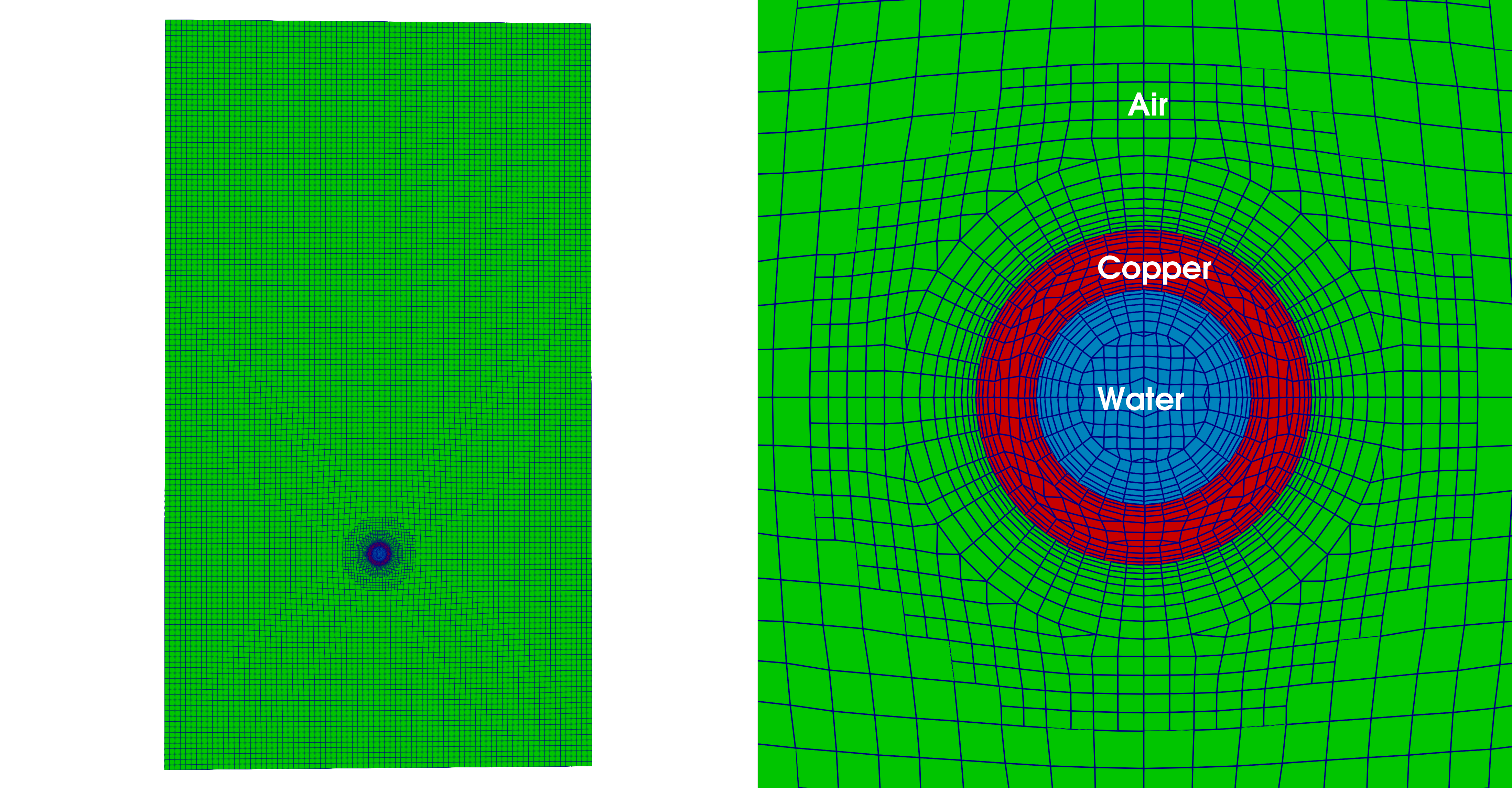
For the needs of this study the quasi-two-dimensional mesh was created in order to make the water flow in the perpendicular direction to x-y plane possible. First, the x-y plane mesh was created, then extruded in z direction. Since the heat transfer is considered (convection from water to copper pipe, conduction through the pipe and convection from the pipe to the surrounding air) it was necessary to create the boundary layer mesh in order to capture thermal boundary layer. Mesh convergence study allowed to choose such mesh density which was the compromise between the simulation time and good accuracy of the results. The final mesh has 130 000 elements which is a good compromise between speed of calculation and accuracy of results.

Parameters of the geometry and physical properties of fluid and solid regions are presented in Table 1.

chtMultiRegionFoam solver was selected for the study. The solver is transient one for buoyant, laminar or turbulent, compressible fluids with radiation models. It is often used for ventilation and heat-transfer phenomena. Two cases were considered: the first one with natural convection and the second one, with forced convection and laminar flow conditions – Reynolds number was 130. For the forced convection case, we were expecting to get characteristic pattern of the wake behind the cylinder, known as von Kármán vortex street. To observe that pattern the simulation was set to 100ms.

The materials applied in the simulation had the following properties - Table 2.

Boundary conditions are very simple and for the case of forced convection, the air inlet was defined as velocity inlet with the velocity equal to 0.0489 [m/s] (together with the pipe diameter it corresponds to Re = 130). The water inlet velocity was set to 5 [m/s]. The outlets are defined as Inlet-Outlet boundary conditions. Remaining surfaces were set to symmetry planes.

Initial conditions were set individually for each region. The air region was initialized from the air inlet, similarly, the water region was initialized from the water inlet.

To capture correctly the wake patterns behind the cylinder, it was necessary to discretize time derivative using backward Euler scheme and the convection term was set to the LUST scheme (which stands for Linear-Upwind stabilized transport), which blends linear upwind with linear interpolation to stabilize solutions while maintaining second-order behaviour.

Figure 2 show temperature contours for the case of a free convection at the Rayleigh number \(Ra = 0.86 \cdot 10^5\). One can observe that the heat from the copper pipe is transferred to the surrounding air. The air around the pipe increases its temperature and due to the density difference a convective flow was induced. The plume behind the cylinder is stable up to several diameters of the pipe. Then instabilities begin and the plume broke up. On the presented result one can observe how the copper pipe is heated by hot water.

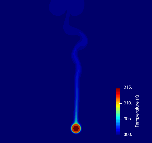
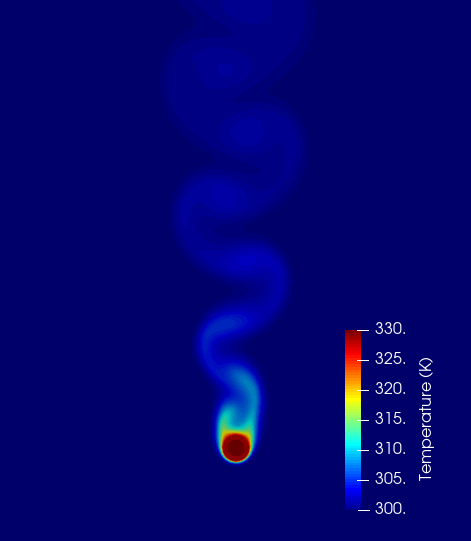
Figure 3 shows temperature contours for the case of a forced convection at \(Re_D = 130\). At this flow regime we can observe the von \(K \acute{a} rm \acute{a} n\) vortex street behind the pipe. The temperature contours depict the vortex street vertical structures. It is the fully developed flow with clear vortices shedding visible behind the copper pipe. Also, the pipe temperature is almost completely equalized with hot water temperature.

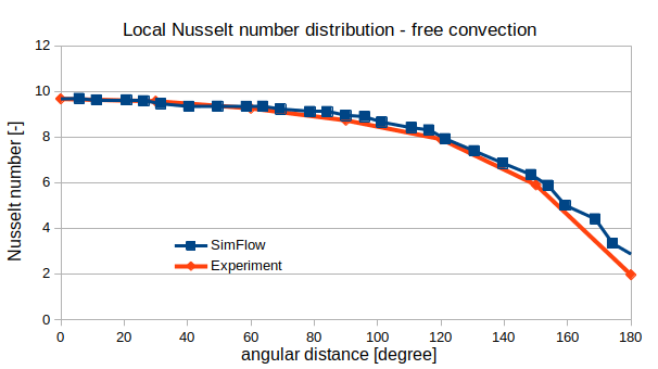
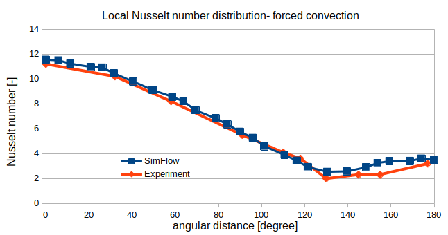
In Figure 4 and Figure 5 the SimFlow results are compared against experimental data [Saitoh et al. (1993)] and <[Eckert and Soehngen. (1952)], respectively for free and forced convection. Zero angle correspond to the upstream stagnation point.

Both distributions, for free and forced convection, show that the maximum Nusselt number occurs at the stagnation point. Heat transfer decreases with angular coordinate to the hot wake. Additionally, for forced convection case, one can observe that at around \(120^\circ\), the minimum is reached. Then, heat transfer increases again due to oscillating wake movement. The agreement with experimental data is very good.

It was proven that SimFlow can predict heat transfer for free and forced convection, including heat exchange between different media. Conjugate heat transfer phenomena can be effectively simulated, not only on the global level, but also local phenomena for the unsteady case. The accuracy of the simulation results was verified against the test data and high fidelity was demonstrated.