Sod Shock Tube Problem - CFD Simulation SimFlow Validation Case

In this article we will study the shock tube problem also known as the Sod problem, investigated deeply by Gary Sod in 1978. By solving the Euler equations we will provide three characteristics, describing the propagation speed of the rarefaction wave, the contact discontinuity and the shock discontinuity. Analytical solution of Sod problem exists, that is why this problem is very often used as a validation case for compressible solvers.

We will investigate 1D numerical simulation of the Sod problem in SimFlow showing high accuracy in solving compressible flows.

The Sod Shock tube is a Riemann problem used to test the accuracy of computational methods. A shock tube consists of a pipe with circular or rectangular cross-section which is filled with a gas. The tube is split into two parts by a diaphragm being positioned in the middle of it - see Figure 1. Numerically, the diaphragm is modeled as a discontinuity in initial fluid conditions (density, pressure and temperature) across this surface.

The initial conditions are very simple for this problem: a contact discontinuity separating gas with different pressure and density, and zero velocity everywhere. In the standard case the density and pressure on the left are unity, The density on the right side of the diaphragm is 0.125 and the pressure is 0.1. The ratio of specific heats is 1.4. The initial conditions can be summarized in the following equation.

where \(\rho\) is density, \(P\) pressure and \(u\) velocity. Indices \(_L\) and \(_R\) refer to left and right-hand side conditions on the side of the diaphragm. By solving the Euler equations we can obtain the time evolution of this problem. As a result we will get three characteristics, describing:

We will compare results from SimFlow to the analytical solution.

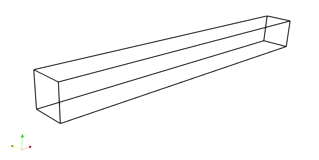
The tube has a rectangular cross-section with dimensions of 0.1mx0.1m and length of 1m. The geometry is presented in Figure 2.

The numerical mesh was created using only the Base Mesh Box tool which is an integral part of SimFlow. It is based on the basic mesh generator available in OpenFOAM that allows creating parametric meshes in a very simple and fast way. Since we are considering 1D case, the mesh in y and z directions contains only 1 cell. For x direction 5000 cells were used.

rhoPIMPLE solver was used to calculate the Sod shock tube problem. This is a pressure-based transient solver for compressible fluid flow. Working fluid is air with thermophysical properties given in Table 1. Please note that dynamic viscosity \(\mu\) is set to \(0\) (as we want to solve Euler equations) and the turbulence modelling is set to laminar. The Prandtl number is not used in this case. As an equation of state we are using ideal gas law.

All boundaries are treated as walls and we apply "zeroGradient" conditions for all flow variables. But for the proper initialization of the model we patched the domain at \(t=0 \; s\) according to equation (1), defining \(p\), \(U\) and \(T\) for left and right-hand sides of the domain. Since we are going to deal with the compressible flow with strong discontinuity like shock waves, the robust and accurate numerical schemes must be considered. Least squares method was used for gradient schemes and limited linear schemes for convective terms. The momentum and energy equations are discretized using PBiCG Stabilized schemes.

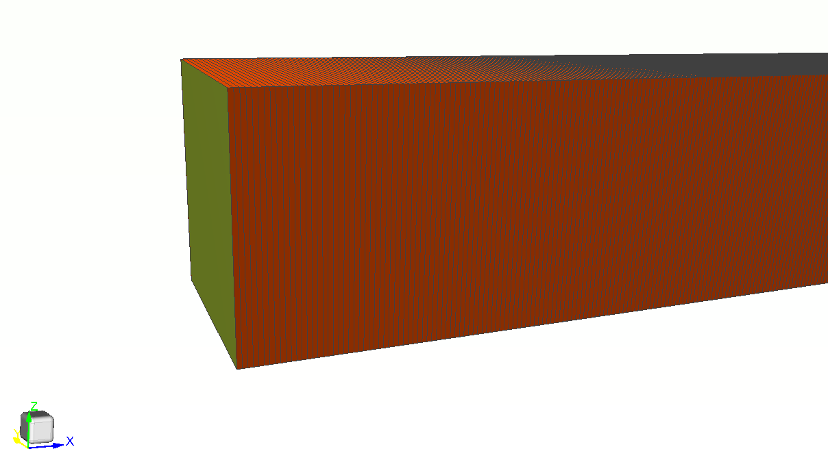
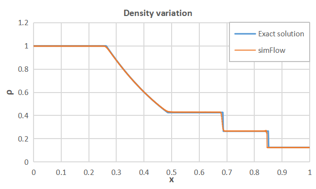
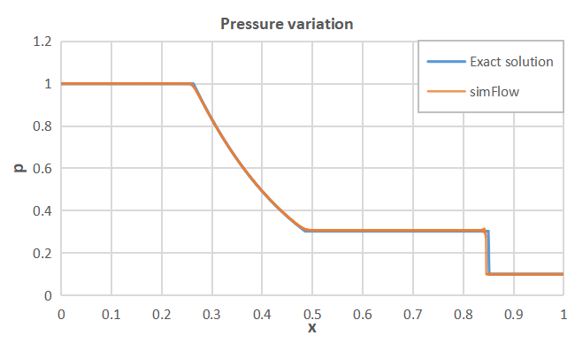
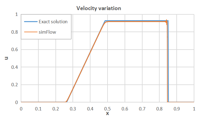
To demonstrate the accuracy of SimFlow we calculated the solution at time \(t=0.2 \; s\) and compare analytical solution to the numerical one by plotting density, pressure and velocity curves along the shock tube.

SimFlow was used to simulate the Sod problem. It was shown that the results obtained are in a very good agreement with the analytical solution. Therefore, SimFlow can be used for modelling of compressible flows with strong discontinuities, providing high quality results.