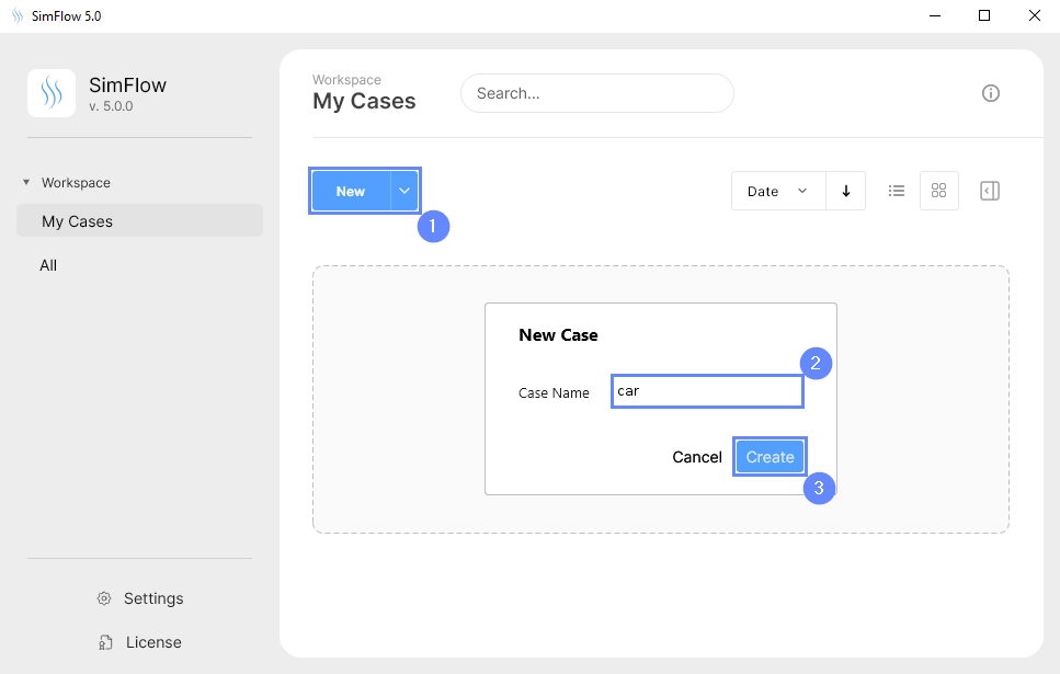
3. Create Case
Open SimFlow and create a new case named car
- Click New
- Provide name car
- Click Create to open a new case
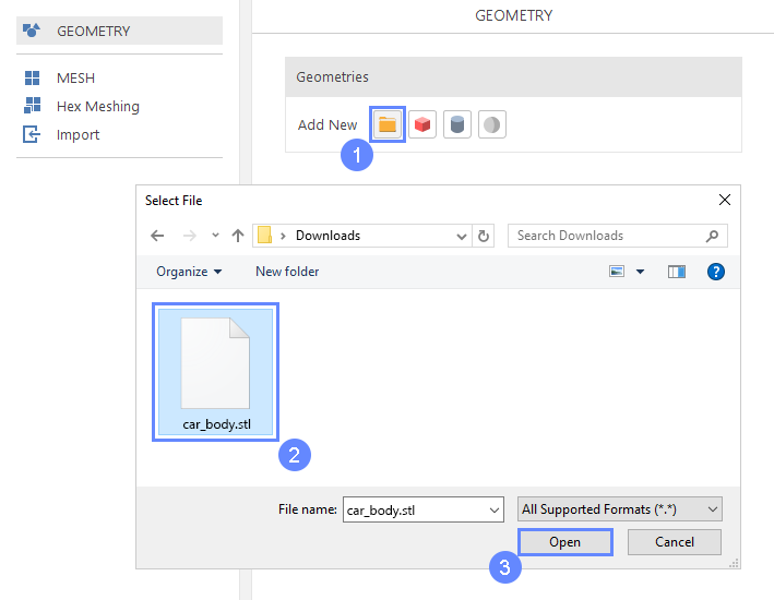
4. Import Geometry
Firstly we need to Download GeometryCar_body
- Click Import Geometry
- Select geometry file car_body.stl
- Click Open
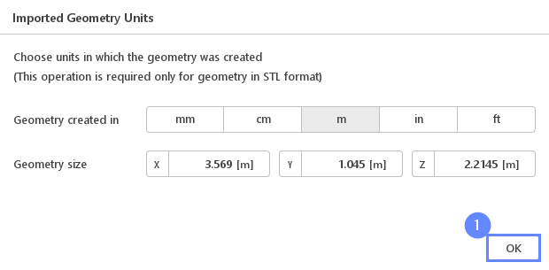
5. Imported Geometry Units
The STL geometry format does not store the unit in which the geometry was created. Geometry size shows the overall size of the model in each direction, what should help to choose the correct unit. In ours case, the default unit meter is correct.
- To confirm default unit meter, press OK
6. Geometry - Car Body
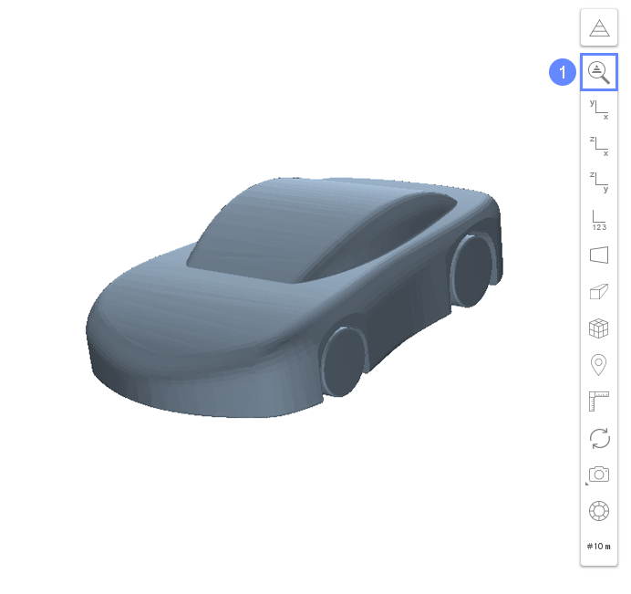
After importing geometry, it will appear in the 3D window
- Click Fit View to zoom in on the geometry
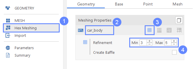
7. Meshing Properties - Car Body
After geometry is loaded, we can proceed to define meshing properties. To better resolve the flow around the car body, we want to refine mesh near the car geometry by specifying minimum and maximum refinement levels.
- Go to Hex Meshing panel
- Select car_body geometry
- Enable Meshing Geometry
- Refine mesh near the surface of the car_body
Refinement Min 3 Max 5
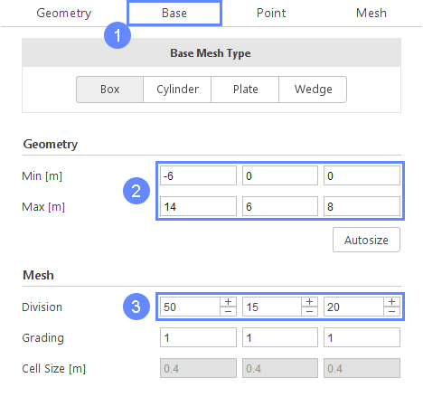
8. Base Mesh
Base Mesh is a domain mesh of our simulation from which the final mesh will be created by carving out the geometry of the car.
- Go to Base tab
- Define base mesh parameters accordingly
Min \({\sf [m]}\)-600
Max \({\sf [m]}\)1468 - Set the division of the base mesh
Division501520
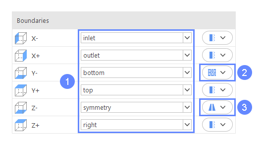
9. Base Mesh Boundaries
We need to assign individual names to each side of the base mesh in order to be later able to define different conditions on each side.
- Define boundary names accordingly
X- inlet
X+ outlet
Y- bottom
Y+ top
Z- symmetry
Z+ right - 3 Define boundary types accordingly
Y- wall
Z- symmetry
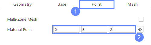
10. Material Point
Material Point tells the meshing algorithm on which side of the geometry the mesh is to be retained. We are modeling car aerodynamics so our material point needs to be located inside the Base Mesh but outside the car body.
- Go to Point tab
- Specify location inside base mesh but outside car geometry
Material Point032
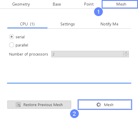
11. Start Meshing
Everything is now set up for meshing
- Go to Mesh tab
- Press Mesh button to start meshing process
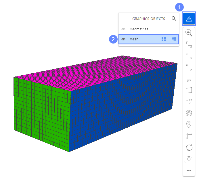
12. Mesh
After meshing is finished, the new mesh will be displayed in the graphics window. To show the mesh of the car body we can use the Graphics Object List.
- Click Graphics Object List icon
- Select Mesh to show meshes list
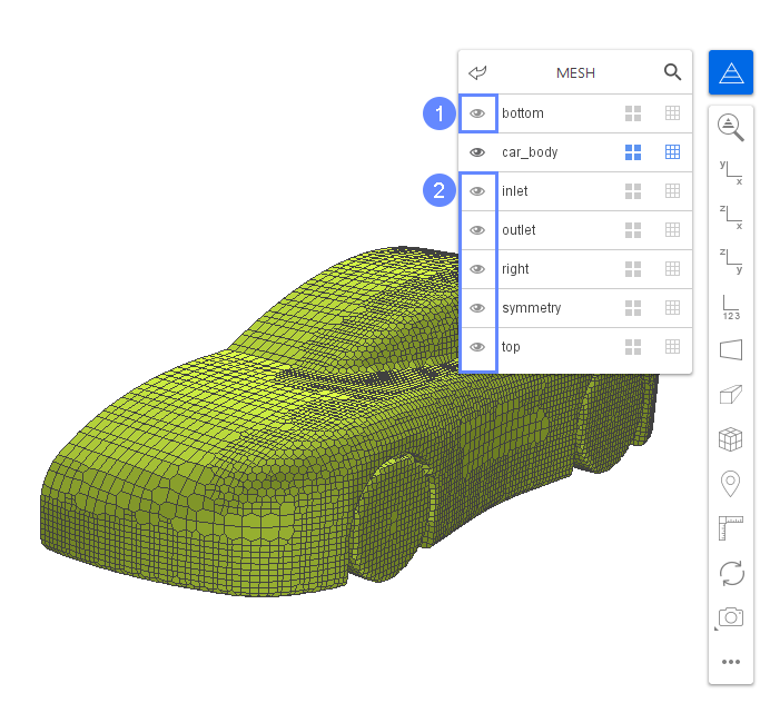
13. Mesh - Toggle Visibility
You can hide domain boundaries to inspect the mesh on the car body.
- 2 Hide the following objects
bottom
inlet
outlet
right
symmetry
top
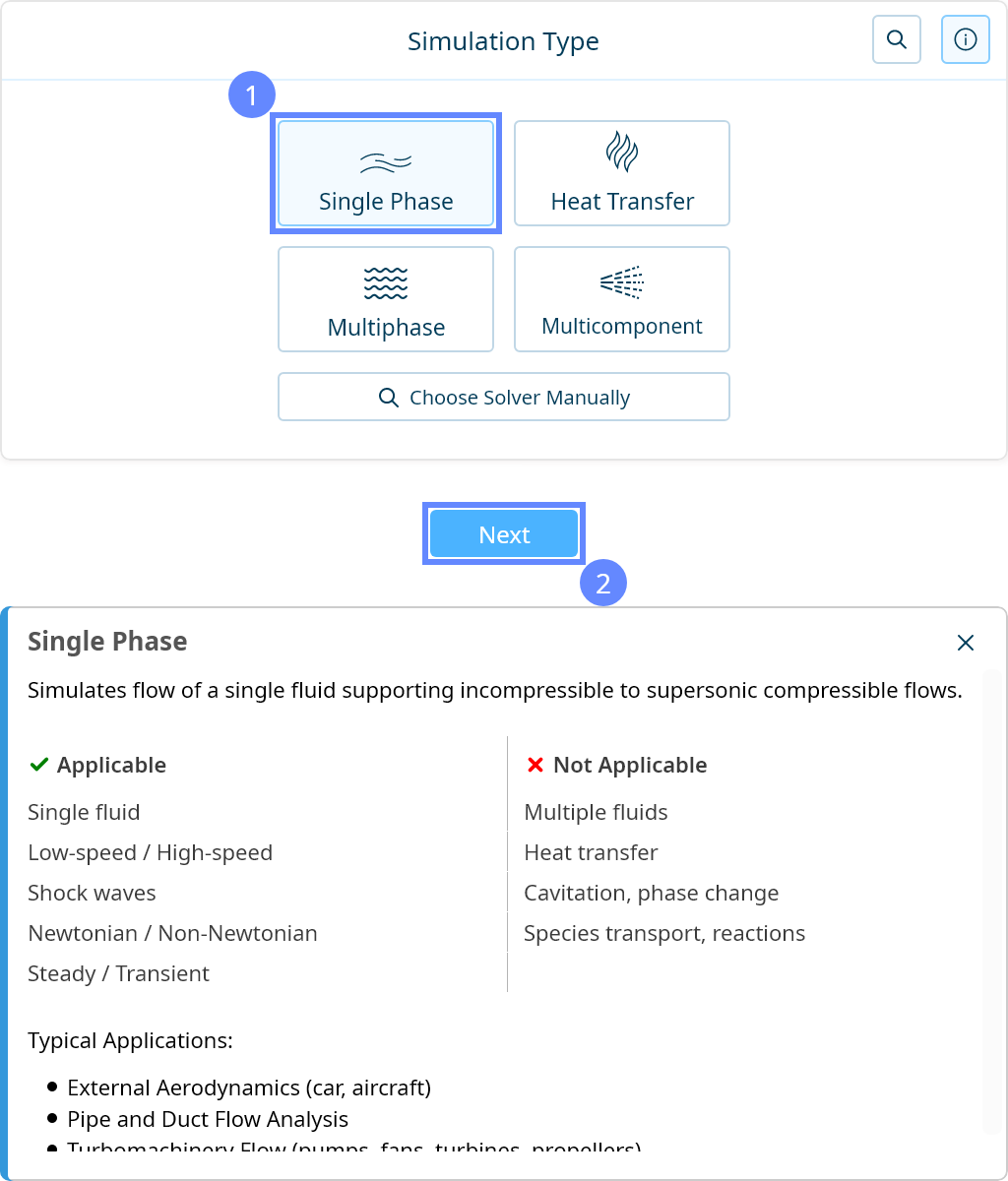
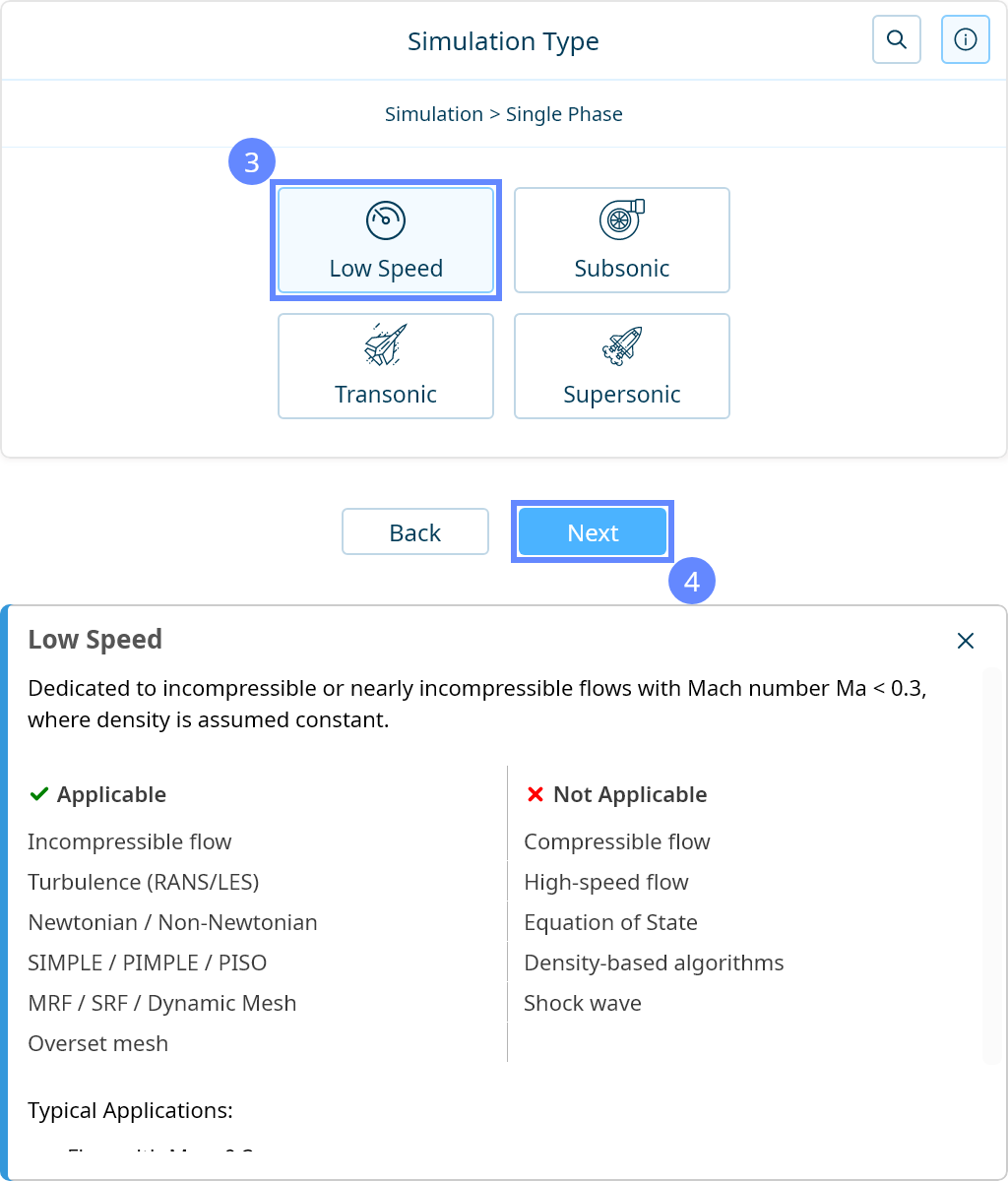
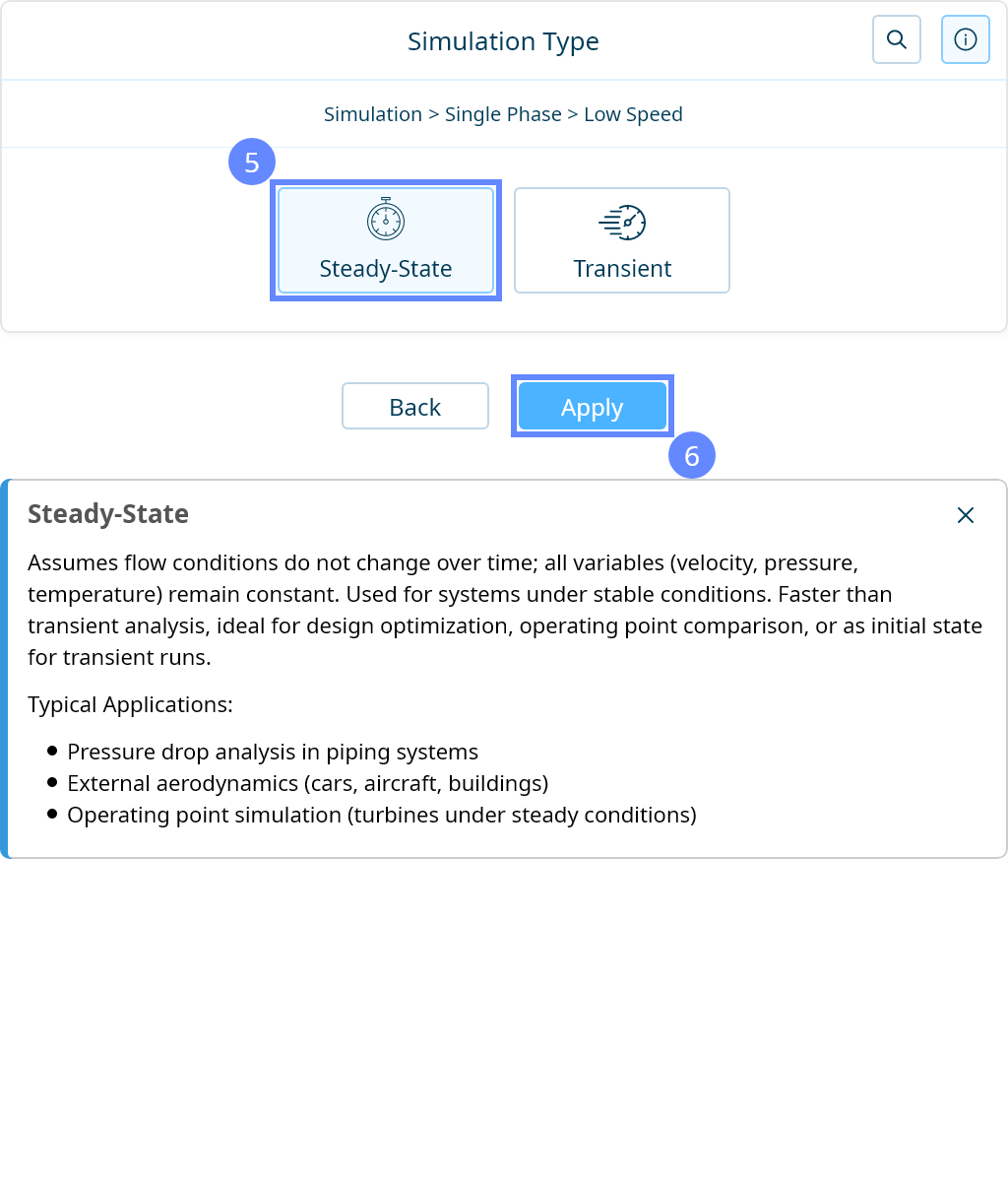
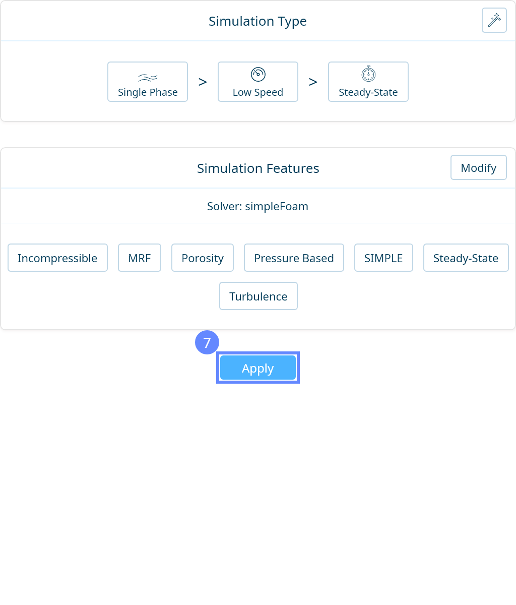
14. Simulation Type
We want to analyze the airflow around the car body. For this purpose, we will use a single-phase, steady-state simulation of incompressible turbulent flow.

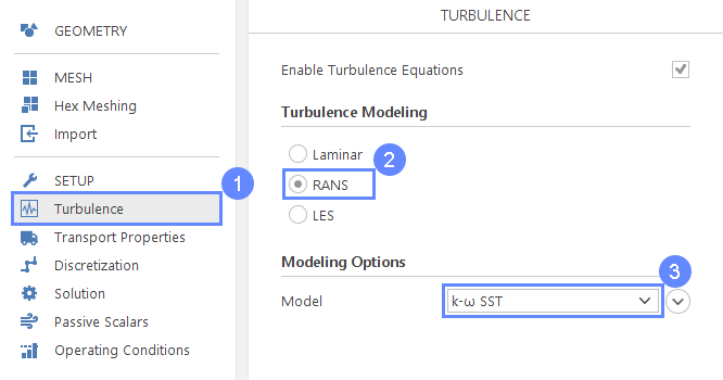
15. Turbulence
We are going to use the standard \(k{-}\omega \; SST\) model to handle turbulence. This model gives very good agreement with experimental data and is commonly used for aerodynamics applications.
- Go to Turbulence panel
- Select turbulence model
Turbulence Modelling RANS - Change default turbulence model
Model \(k{-}\omega \; SST\)
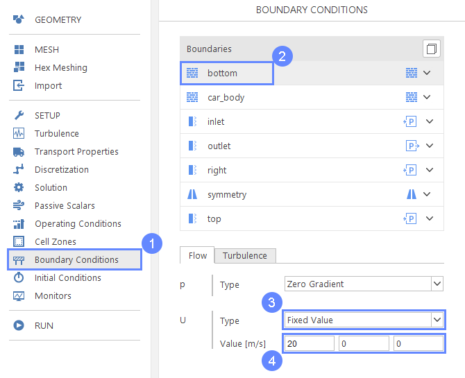
16. Boundary Conditions - Bottom (Flow)
We are simulating a car moving on a road. In this reference frame, the road has to move with respect to the car. We can achieve this by applying fixed velocity boundary condition on the bottom of the domain.
- Go to Boundary Conditions panel
- Select bottom boundary
- 4 Set velocity
UTypeFixed Value
UValue \({\sf [m/s]}\)2000
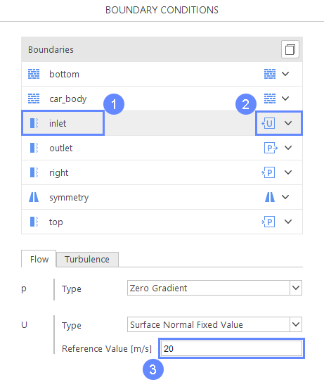
17. Boundary Conditions - Inlet (Flow)
On the inlet, we are going to apply constant velocity, similarly to the bottom .
- Select inlet boundary
- Change boundary character
inlet Velocity Inlet - Define inlet velocity
UReference Value \({\sf [m/s]}\)20
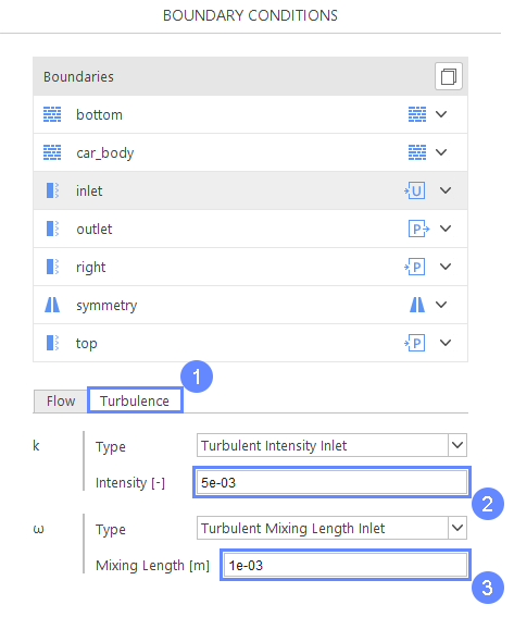
18. Boundary Conditions - Inlet (Turbulence)
We are simulating a car moving in otherwise stationary air. Therefore, we specify low turbulence intensity on the inlet.
- Go to Turbulence boundary conditions tab
- 3 Set the following parameters accordingly
kIntensity \({\sf [-]}\)5e-03
\(\omega\)Mixing Length \({\sf [m]}\)1e-03
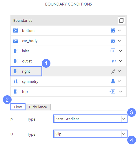
19. Boundary Conditions - Right (Flow)
On the right and top boundary, we are going to force velocity to be tangent to the boundary.
- Select right boundary condition
- Go to Flow tab
- 4 Define slip wall condition
TypepZero Gradient
TypeUSlip
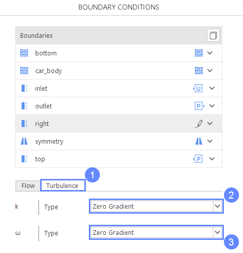
20. Boundary Conditions - Right (Turbulence)
- Go to Turbulence tab
- 3 Change turbulent kinetic energy and frequency types to
TypekZero Gradient
Type\(\omega\)Zero Gradient
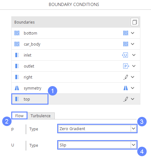
21. Boundary Conditions - Top (Flow)
We need to repeat the same steps to the top boundary condition
- Select top boundary condition
- Go to Flow tab
- 4 Define slip wall condition
TypepZero Gradient
TypeUSlip
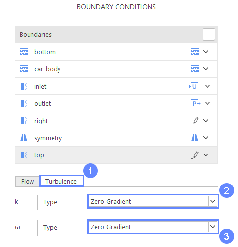
22. Boundary Conditions - Top (Turbulence)
- Go to Turbulence tab
- 3 Change turbulent kinetic energy and frequency types
TypekZero Gradient
Type\(\omega\)Zero Gradient
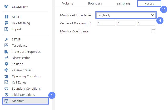
23. Monitors - Forces
We want to monitor the simulation process by observing plots of the aerodynamic forces on the car
- Go to Monitors panel
- Go to Forces tab
- Enable observing forces on the car_body boundary
Monitored Boundaries car_body
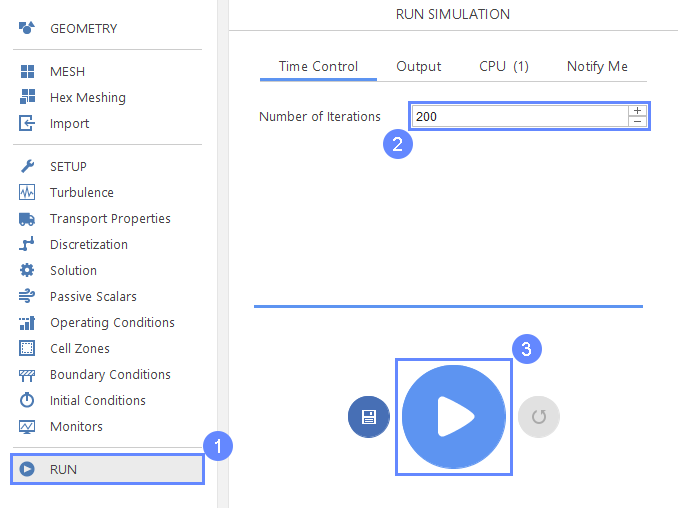
24. Run Simulation
- Go to Run panel
- Set maximal number of iteration that solver can perform before stopping
Number of Iterations200 - Click Run Simulation button
Estimated computation time: 20 minutes
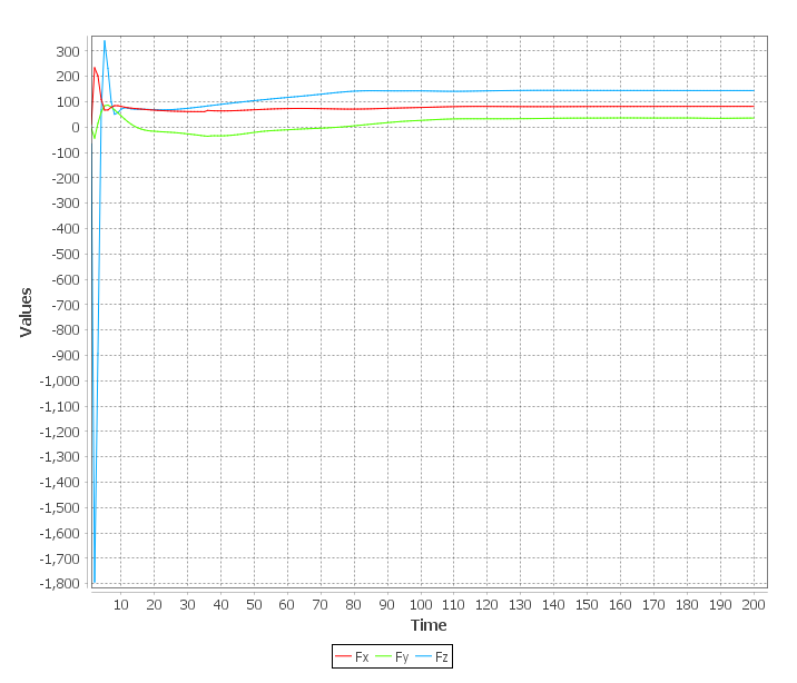
25. Monitor Forces
During the simulation, we can observe whether forces on the car body stabilize which will mean that our simulation converges
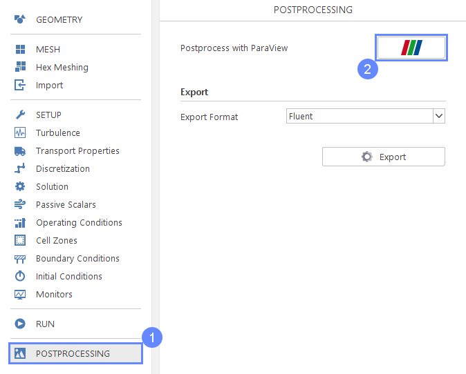
26. Postprocessing - ParaView
After the simulation is finished, we can proceed to post-processing
- Go to Postprocessing panel
- Start ParaView
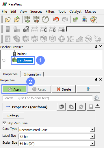
27. ParaView - Load Results
- Make sure you have your case selected car.foam
- Click Apply to load results
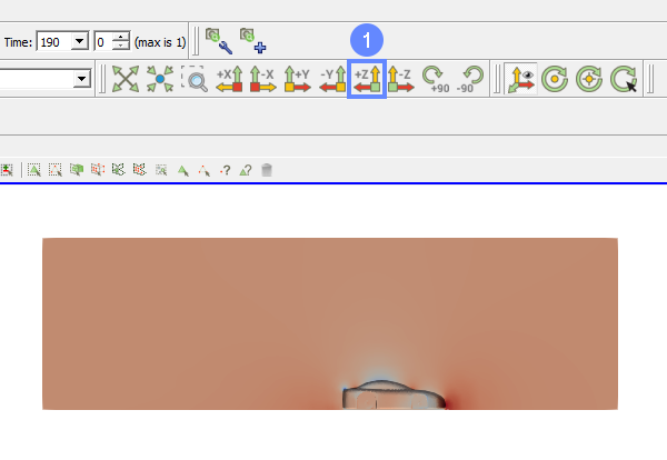
28. ParaView - Set View Direction
After loading results, we have to rotate the domain or change view direction to see the car.
- Click Set view direction to +Z
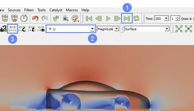
29. ParaView - Display Velocity
We will now display velocity (U) contours.
- Load latest results by clicking Last Frame icon
- Select U (velocity) from the dropdown menu
- Click Rescale to data range
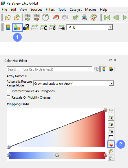
30. ParaView - Coloring (I)
We can change the coloring scheme in ParaView to have nicer colors.
- Click Edit Color Map from the menu placed on the left side, if the panel is not already shown.
- Select Choose Preset from the Color Map Editor placed by default on the right side of the ParaView
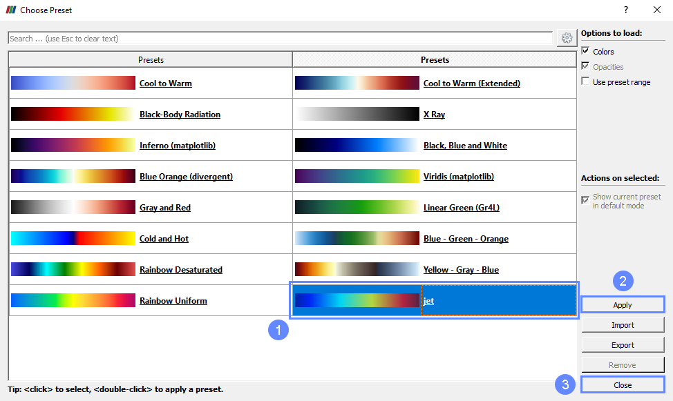
31. ParaView - Coloring (II)
We can now select a new Color Preset.
- Select jet preset
- Apply changes
- Close the window
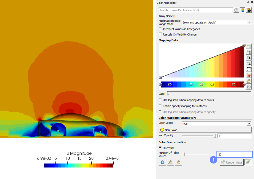
32. ParaView - Coloring (III)
Now we can see the results with the new preset applied. We can also modify the number of displayed colors to see the results better.
- Decrease color scale resolution to make velocity regions more distinguishable (non-smooth color transition)
Number of Table Values 20
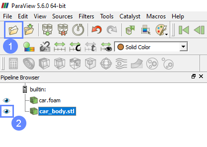
33. ParaView - Import Geometry
To display results on the original geometry, we can import the geometry directly into ParaView.
- Click Open and select the original car_body.stl geometry to import it into ParaView.
- Click on the Visibility icon to show the geometry.
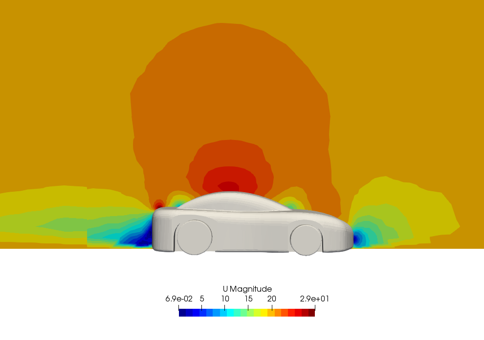
34. ParaView - Final Results
Now we can see the final results with the original geometry.
