Introduction
Natural convection phenomena are often encountered in many practical applications, from simple domestic situations like room heating to industrial and nuclear installations. Though the process seems to be simple, in fact it might be very complex. Mostly because in such a heated cavity that we are going to consider, at the same time we will find regions of fully turbulent flow and regions of low turbulent Reynolds number. It is also possible to find in such situations regions of laminar flow or even regions of stagnation. Because of these reasons, simple turbulence modelling of such flows with standard near wall treatment may not give accurate results.
In this article we will conduct a numerical simulation that replicates the experiment of [Betts et al. (2000)]. We will model the rectangular cavity in SimFlow and set the temperature difference between two vertical walls at \(19.6^oC\) and \(39.9^oC\), resulting in Rayleigh number (based on the width) of \(0.86 \cdot 10^6\) and \(1.43 \cdot 10^6\). At the end of the article we will compare numerical results to the test data available on [ERCOFTAC database] to demonstrate high accuracy and predictability of SimFlow.
Geometry and numerical mesh
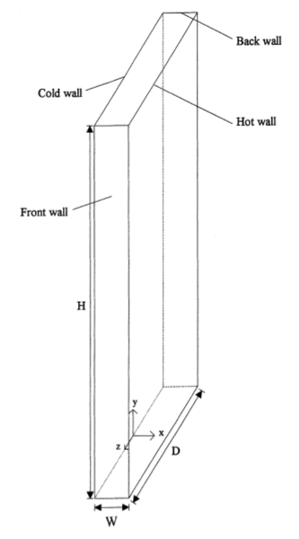
The geometry of the cavity is cuboid with dimensions H x W x D being: 2.18m x 0.076m x 0.52m - Figure 1.
The numerical mesh was created in Box Base Mesh utility which is an integral part of SimFlow. It is a very basic mesh generator available in OpenFOAM that allows creating parametric meshes in a very simple and fast way. For meshing the cavity the tool is very useful and sufficient.
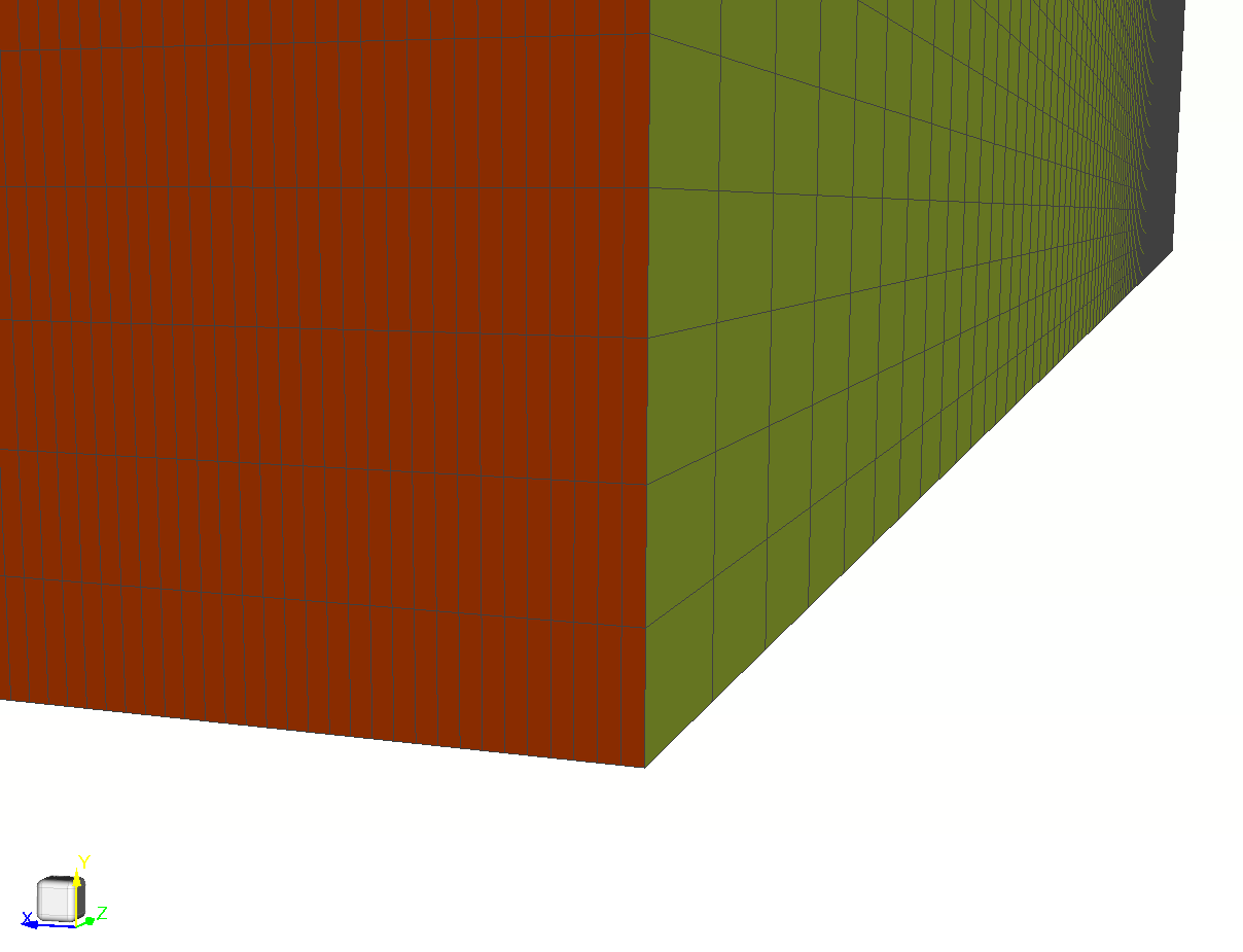
Mesh convergence studies were performed in order to define the most optimal mesh density. The final mesh consists of 11 million cells, with uniform grading applied in x, y and z directions.
The mesh details are presented in Figure 2.
Model setup and boundary conditions
Buoyant Simple solver was selected to model the flow in the cavity. The solver is dedicated to model steady-state, compressible flows with buoyancy and turbulence phenomena.
Working fluid is air with thermophysical properties given in Table 1. Perfect gas equation of state was used.
| \(M \; [\frac{g}{mol}]\) | \(C_p \; [\frac{J}{kg \cdot K}]\) | \(\mu \; [Pa \: s]\) | \(P_r \; [-]\) |
|---|---|---|---|
\(28.96\) | \(1005\) | \(1.8\cdot 10^{-5}\) | \(0.7\) |
\(k{-}\omega\) turbulence model was selected for the validation. Since \(y^+\) values varies between less than 1 up to 5 low Re wall function treatment was used. All domain boundaries are wall type boundary conditions. The exact set-up of boundary conditions is presented in Table 2.
| Boundary Type | Cold Wall | Hot Wall | Top and bottom walls | Front and back walls |
|---|---|---|---|---|
Velocity | \(0 \; [\frac{m}{s}]\) | \(0 \; [\frac{m}{s}]\) | \(0 \; [\frac{m}{s}]\) | \(0 \; [\frac{m}{s}]\) |
Modified pressure | Fixed Flux Pressure | Fixed Flux Pressure | Fixed Flux Pressure | Fixed Flux Pressure |
Temperature | \(288.15 \; [K]\) | \(307.75/328.05 \; [K]\) | Zero Gradient | Zero Gradient |
k | \(0 \; [\frac{J}{kg}]\) | \(0 \; [\frac{J}{kg}]\) | \(0 \; [\frac{J}{kg}]\) | \(0 \; [\frac{J}{kg}]\) |
\(\omega\) | Standard Wall Function | Standard Wall Function | Standard Wall Function | Standard Wall Function |
\(\nu\) | Low Re Wall Function | Low Re Wall Function | Low Re Wall Function | Low Re Wall Function |
\(\alpha\) | Standard Wall Function | Standard Wall Function | Standard Wall Function | Standard Wall Function |
Both, momentum and turbulence transport equations were discretized using Linear second order accuracy scheme.
GAMG linear solver was used for pressure and PBiCGStab with DILU preconditioner for velocity and turbulence. Very small value of tolerance was used for all equation, at the level of 1e-08 for pressure and 1e-15 for velocity and turbulence.
SimFlow allows plotting the residuals and selected monitors on-the-run. In this case we concluded that solution is converged when residuals were at the level 1e-06 and monitored fluid variables were constant.
Results
Simulations were performed for two different Rayleigh number. Rayleigh number is described by the equation:
\(Ra_x=\frac{g \beta }{\nu \alpha} (T_s - T_{\infty})x^3\)
where:
- \(Ra_x\) - is the Rayleigh number for characteristic length x
- \(x\) - is the characteristic length
- \(g\) - is acceleration due to gravity
- \(\beta\) - is the thermal expansion coefficient
- \(\nu\) - is the kinematic viscosity
- \(\alpha\) - is the thermal diffusivity
- \(T_s\) - is the surface temperature
- \(T_{\infty}\) - is the quiescent temperature (fluid temperature far from the surface of the object)
We modeled the rectangular cavity in SimFlow and set the temperature difference between two vertical walls at \(19.6^oC\) and \(39.9^oC\), resulting in Rayleigh number (based on the width) of \(0.86 \cdot 10^6\) and \(1.43 \cdot 10^6\).
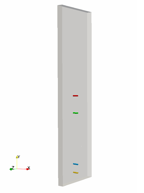
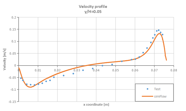
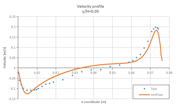
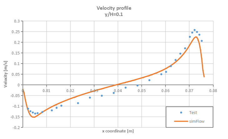
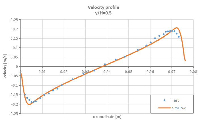
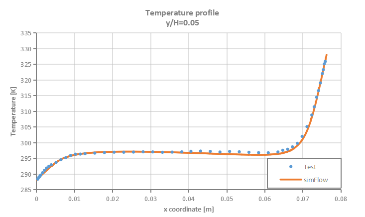
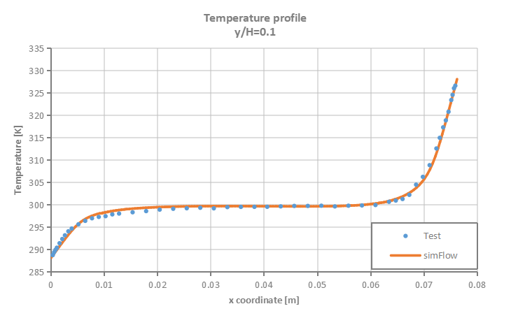
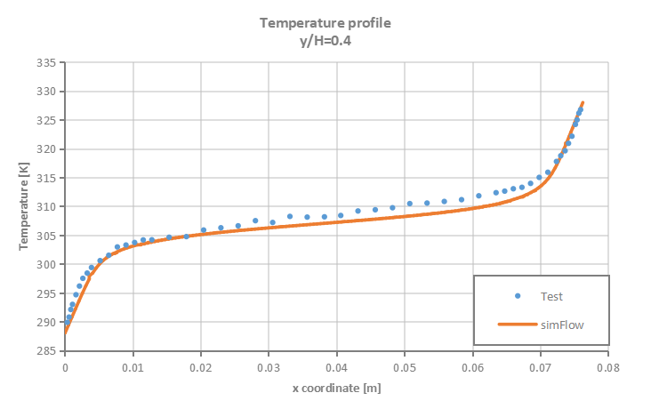
Velocity and temperature profiles are plotted at selected section cuts of the domain as presented in Figure 3 and then compared to test data.
- Low Rayleigh number \(0.86 \cdot 10^6\)
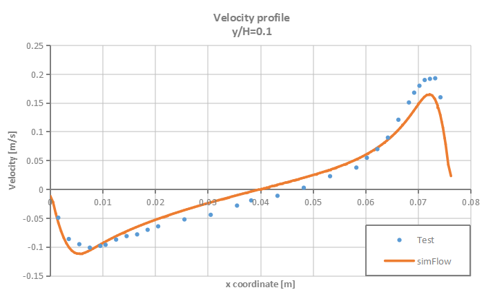
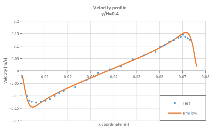
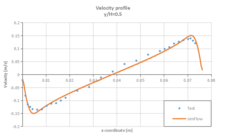
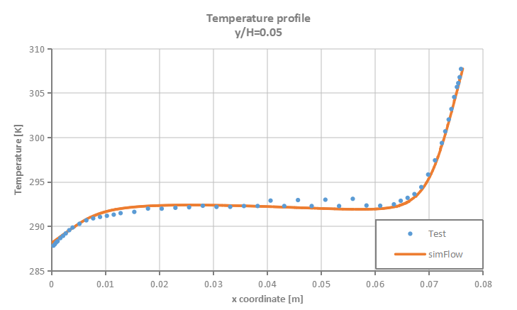
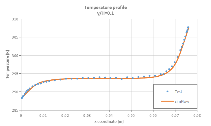
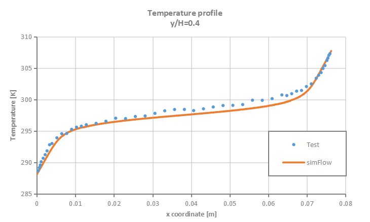
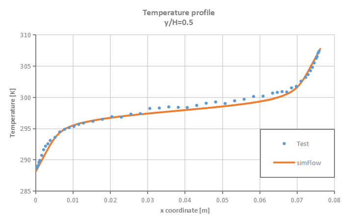
- High Rayleigh number \(1.43 \cdot 10^6\)


Summary
SimFlow was used to simulate natural convection process in enclosed cavity with two vertical heated walls. The accuracy of the simulation results was verified against the test data. It was proven that SimFlow is capable of predicting with high accuracy buoyancy driven flows.
Literature
- [Betts et al. (2000)] Betts, P L & Bokhari, H I 2000, "Experiments on turbulent natural convection in an enclosed tall cavity", International Journal of Heat and Fluid Flow, vol. 21, pp. 675-683
- [ERCOFTAC database] ]ERCOFTAC database: Turbulent Natural Convection in an Enclosed Tall Cavity http://cfd.mace.manchester.ac.uk/ercoftac/doku.php?id=cases:case079